A multi-scale convolutional Siamese network for few-shot fault diagnosis of unmanned aerial vehicle rotor

Han, Tubao; Du, Canyi; Yang, Xiaoqing; Huang, Yongxian; Zeng, Xiangkun; Yu, Feifei; Gong, Yongkang; Zhang, Junyi; Zhou, Wenzhu; Qi, Jie

doi:10.21595/jve.2025.25101

Journal of Vibroengineering

Browse Journal

Submit article

Published: December 14, 2025

Check for updates

A multi-scale convolutional Siamese network for few-shot fault diagnosis of unmanned aerial vehicle rotor

Tubao Han¹

Canyi Du²

Xiaoqing Yang³

Yongxian Huang⁴

Xiangkun Zeng⁵

Feifei Yu⁶

Yongkang Gong⁷

Junyi Zhang⁸

Wenzhu Zhou⁹

Jie Qi¹⁰

^{1, 2, 3, 4, 5, 7, 8, 9, 10}School of Automobile and Transportation Engineering, Guangdong Polytechnic Normal University, Guangzhou, 510665, People’s Republic of China

⁶School of Electromechanical Engineering, Guangdong Polytechnic Normal University, Guangzhou, 510665, People’s Republic of China

Corresponding Author:

Canyi Du

Cite the article Download PDF

Article in Press

Downloads 0

Abstract

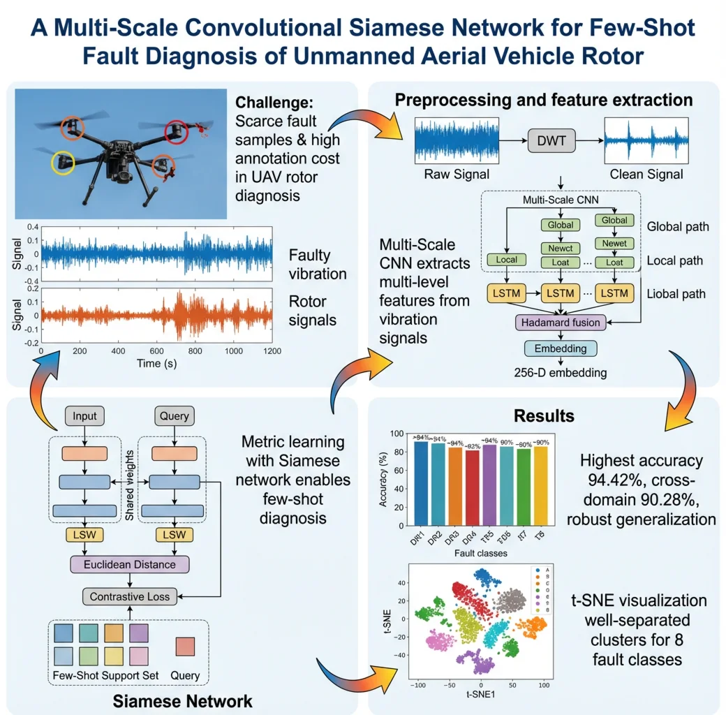
Unmanned Aerial Vehicles (UAVs) often face infrequent fault occurrences and high manual annotation costs, resulting in a critical shortage of valid fault samples for diagnostic research. Traditional fault diagnosis methods struggle with small sample sizes. This paper proposes a novel deep metric learning method, the Multi-Scale Convolutional Siamese Network (MSCSN), to address the few-shot learning problem in UAV rotor fault diagnosis. First, discrete wavelet transform (DWT) is used to compress and normalize the vibration signals, enhancing the prominence of signal features. Then, based on the multi-scale convolutional neural network (MS-CNN) model, the network automatically extracts multi-level features from rotor fault vibration signals, improving its adaptability to complex data. Finally, the Siamese network structure, with shared parameters and identical architecture, processes sample pairs and incorporates a small number of support samples for few-shot learning. Experimental results show that the proposed model achieves a highest accuracy of 94.42 % in few-shot tasks. In cross-domain transfer learning tests, the model achieves an average accuracy of 90.28 %, demonstrating its superior generalization ability and robustness across different environments. We also validated the model's stability using the publicly available MVS-UAV-BF dataset.

1. Introduction

Technology has been a key driver of globalization, with Unmanned Aerial Vehicles (UAVs) being increasingly adopted across various sectors such as military, healthcare, and agriculture. UAV fault diagnosis technology is critical for improving system reliability, ensuring safety during flight, and minimizing unnecessary costs. In recent years, fault diagnosis techniques have seen significant advancements [1]-[4].

In intelligent UAV fault diagnosis, machine learning and early deep learning methods have achieved promising results. Chen et al.[5] developed a UAV sensor fault diagnosis approach based on a BP neural network combined with a genetic algorithm. Gino Iannace [6]constructed a decision-tree-based classification model using UAV-generated noise measurements to detect imbalanced rotor blades. Chen et al. [7]replaced traditional shallow neural networks with deep belief networks (DBNs) trained on a large dataset to enable early fault warnings. Yang et al. [8]proposed a UAV fault pattern recognition method using sequential information fusion and support vector machines.

With the rise of deep learning, fault diagnosis has been significantly enhanced, eliminating the need for time-consuming manual analysis. Techniques like Convolutional Neural Networks (CNN) [9]-[13] and Long Short-Term Memory networks (LSTM) [14]-[16] effectively extract fault information but typically require large amounts of training data. However, in practical industrial settings, fault data is often limited, and labeled samples are scarce. Recent studies have focused on diagnosing faults with limited data. For instance, Chen et al. [16] proposed a hybrid neural network model combining width learning and CNN, which showed promising results in few-shot fault diagnosis. Hang et al. [17]applied Principal Component Analysis (PCA) to handle imbalanced fault diagnosis data, and Duan et al. [18] introduced the Support Vector Data Description (SVDD) method for dealing with imbalanced datasets. Recently, deep neural networks leveraging few-shot learning have gained traction for solving data scarcity issues and have been applied in areas such as intelligent agriculture [19], image classification [20], [21], incremental learning [22], and mechanical fault diagnosis [23]-[25].

Despite the success of few-shot learning in fault diagnosis, its application to UAV fault diagnosis has been limited. To tackle the problem of diagnosing UAV faults with limited samples, this paper introduces a Multi-Scale Convolutional Siamese Network (MSCSN), using metric learning to achieve effective rotor fault diagnosis in few-shot scenarios. The contributions of this paper are as follows:

1) Multi-Scale convolutional neural network automatically extracts feature representations from UAV rotor fault vibration signals using convolutional neural networks at different scales, effectively capturing multi-level signal features.

2) Siamese network enhances generalization through pair generation and feature comparison, while the contrastive loss function drives similar samples to cluster and dissimilar samples to separate, further improving the accuracy of fault diagnosis.

3) Exact fault types of drone rotors are automatically diagnosed by leveraging vibration signals through a Siamese network-based metric learning algorithm, overcoming data scarcity without requiring additional frequency analysis. When considering the challenges in UAV fault diagnosis, such as the necessity for cross-domain fault identification.

2. Related work

In recent years, hybrid approaches that combine deep learning with mathematical modeling or signal processing have been increasingly applied to unmanned aerial vehicle fault diagnosis. Among mathematical models, state observer-based methods are commonly used, especially when data augmentation is needed. A well-known technique in this category is filtering, which relies on the dynamic equations of the system being analyzed. By processing these equations, the key harmonic components in generated signals can be identified. In fault detection systems, control signal filtering is commonly employed for diagnosis. Xu et al. [26] proposed a Physics-Informed Probabilistic Deep Network (PIPDN) that integrates physical priors into the loss function while quantifying uncertainty, thus improving reliability in fault diagnosis. Lai et al. [27] developed a Physics-Informed Deep Autoencoder for fault detection in newly designed systems, embedding physical laws into training to enhance detection under small-sample and weakly labeled conditions. Zarchi et al. [28] presented an adaptive physics-guided hybrid diagnostic method combining physics-based feature libraries with evolutionary optimization for cross-condition fault identification. The establishment of precise physical models is a necessary prerequisite for diagnosis. However, building accurate physical models for UAVs is both difficult and time-consuming. Moreover, when fault diagnosis is required for different UAVs, the constructed models are often not reusable.

Signal-based techniques such as the Fast Fourier Transform (FFT) and its variants are still dominant, but decomposition methods and signal envelope analysis are gaining attention due to their excellent feature extraction capabilities. These approaches bridge the gap between traditional signal processing and deep learning techniques. Xu et al. [29] proposed LTFAFormer, a lightweight Transformer architecture capable of robust bearing fault diagnosis in high-noise environments, suitable for industrial deployment. Yuan et al. [30] introduced the IWOA-VMD-KELM pipeline, achieving high accuracy on CWRU and SEU datasets. Jiang et al. [31] presented a parallel TCN-Transformer hybrid model, capturing both local temporal features and global dependencies for improved diagnostic accuracy. These methods have achieved notable results; however, selecting appropriate signal processing techniques and extracting suitable signal features often requires researchers to possess extensive knowledge and expertise. Although this approach is highly popular among researchers, it raises the threshold for practical application.

In the field of intelligent fault diagnosis, researchers have proposed various few-shot learning methods to address the issue of sample scarcity, including meta-learning, data augmentation, and metric learning. Li et al.'s Meta-Feature Enhancement Meta-Learning (MFEML) [32] for bearing fault identification across different rigs, and Luo et al. Elastic Prototypical Network (EProtoNet) [33] for unstable-speed fault diagnosis. Tang et al. [34] proposed a prior-knowledge-enhanced self-supervised framework using time–frequency invariance, reducing labeled data needs while improving cross-condition transfer. Pan et al. [35] proposed CWDAN-SCL, integrating supervised contrastive learning with a complementary weighted dual-adversarial network for open-set domain-adaptive fault diagnosis.

Metric learning approaches – particularly Siamese networks optimized with contrastive or triplet objectives – have become a mainstay for few-shot fault diagnosis because they learn an embedding in which intra-class samples are close while inter-class samples are separated by a margin. Their pairwise (or episodic) formulation effectively amplifies scarce labels by generating $ο (N^{2})$ training pairs from $N$ samples, easing data scarcity and class imbalance. In vibration-based diagnosis, Siamese models are also attractive for cross-condition generalization: once a stable metric space is learned, novel classes or operating conditions can be handled with lightweight support sets and nearest-neighbor classification, avoiding full model retraining. Nevertheless, many existing Siamese pipelines rely on single-scale convolutional encoders or hand-crafted features, which may under-represent multi-frequency, transient, and long-range temporal patterns that are characteristic of UAV rotor signals. These limitations motivate a multi-scale, sequence-aware encoder coupled with a simple metric objective. The Principle of Metric Learning Based on Siamese Networks in Fig. 1. By inputting a pair of samples (such as images) into a shared-parameter feature extractor, their feature representations are extracted, and then their distance or similarity is computed to determine whether they belong to the same or different categories.

Fig. 1The principle of metric learning based on Siamese networks

Building on the above, we adopt a Siamese architecture trained with a contrastive loss while designing a Multi-Scale CNN encoder augmented with LSTM-based temporal modeling. Two parallel convolutional paths capture complementary global (low-frequency, long-range) and local (high-frequency, transient) attributes; element-wise feature fusion yields a compact embedding used with Euclidean distance at test time for support-query matching. This design preserves the label efficiency and generalization of metric learning while better aligning the encoder with the spectral-temporal structure of rotor vibrations. In Section 3 we formalize the metric and loss, and in Section 4 we introduce the experimental setup, fault configuration, and datasets used for model evaluation. In Section 5 we analysis the performance of the MSCSN model in few-shot experiments, cross-condition experiments, and in Section 6 we conclude the paper and outlines future research directions.

3. Proposed method

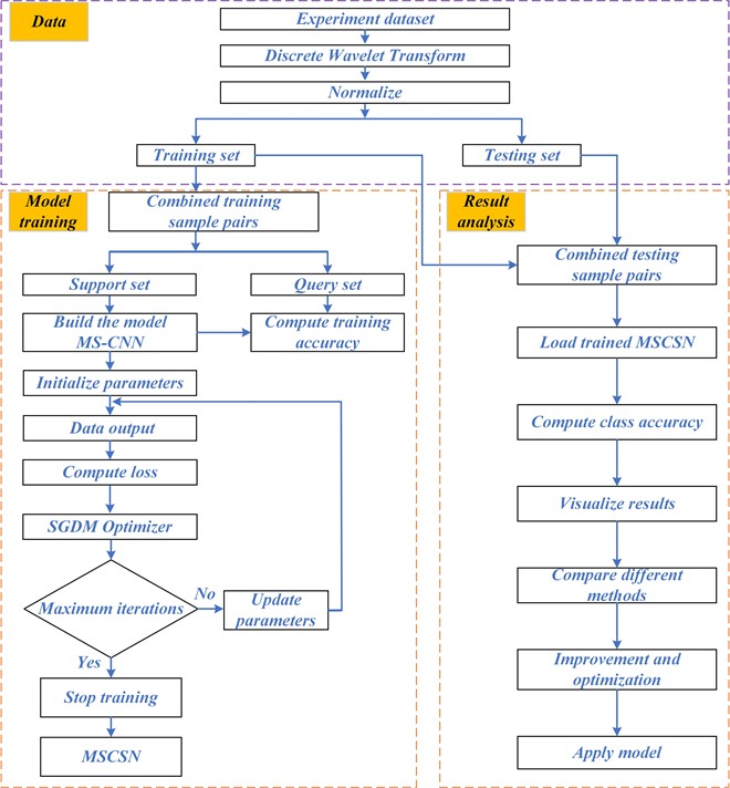
This paper proposes a diagnostic model, MSCSN, combining Multi-Scale Convolutional Neural Networks (MS-CNN) with Siamese Networks to address the issue of sample scarcity in UAV rotor fault diagnosis. The model is designed to solve the fault classification problem with limited training samples by integrating signal resampling, multi-scale feature extraction, and metric learning. The overall diagnostic steps are shown in Fig. 2, which consists of five phases: data preprocessing, feature extraction, metric learning, classification, and fine-tuning. To enhance reproducibility, the theoretical motivations for design choices are elaborated below.

Fig. 2Diagnostic steps of the MSCSN method

3.1. Preprocessing module

Raw vibration signals are acquired at 1024 Hz. To ensure timely inference while retaining discriminative content, each sample spans two rotor cycles and is then compressed using a two-level discrete wavelet transform (DWT) with Daubechies db4; only the approximation coefficients are retained, yielding a 1-D sequence of length 512 (each DWT level halves the length from 2048 to 1024 to 512). Specific procedure:

Step 1: We select db4 as the compression scheme.

Step 2: Perform a two-level discrete wavelet decomposition on the signal:

1

x (t) = \sum_{k} c_{j} [k] ϕ_{j, k} (t) + \sum_{j = 1}^{J} \sum_{k} d_{j} [k] ψ_{j, k} (t),

2

c_{j} [k] = \sum_{n} h [n - 2 k] c_{j - 1} [n],

3

d_{j} [k] = \sum_{n} g [n - 2 k] c_{j - 1} [n],

4

{\tilde{x}}_{i} = \{c_{j} [k], d_{j} [k], d_{j - 1} [k], \dots, d_{1} [k]\} .

Step 3: To align with the learning mechanism of neural networks, we further normalize the compressed signal:

5

x_{i}^{*} = \frac{{\tilde{x}}_{i} - \min (\tilde{x})}{\max (\tilde{x}) - \min (\tilde{x})}, x_{i}^{*} \in [0,1],

6

x_{i}^{*} = \frac{{\tilde{x}}_{i} - μ}{σ},

7

μ = \frac{1}{N} \sum_{i = 1}^{N} {\tilde{x}}_{i},

8

σ = \sqrt{\frac{1}{N} \sum_{i = 1}^{N} ({\tilde{x}}_{i} - μ)^{2}} .

In Table 1, we explain the parameters involved in the above signal processing procedure. After preprocessing, the data are split for few-shot learning: per class, a small subset forms the training/support pool, and the remainder forms the test/query pool; pairs are down sampled to balance positive and negative pairs.

Table 1Parameters involved in the signal processing process

Symbol	Parameter	Description
$c_{j} [k]$	Wavelet coefficients	Wavelet coefficients
$d_{j} [k]$	Wavelet detail coefficients	Wavelet detail coefficients
$ϕ_{j, k} (t)$	Scaling function	Scaling function for DWT
$ψ_{j, k} (t)$	Wavelet function	Wavelet function for DWT
$h [n]$	Approximation filter	Filter used for approximation coefficients
$g [n]$	Detail filter	Filter used for detail coefficients
${\tilde{x}}_{i}$	Normalized value	Normalized values of the data
$μ$	Mean	Mean of the data
$σ$	Standard deviation	Standard deviation of the data
$\max (\tilde{x})$ , $\min (\tilde{x})$	Max value	Maximum value of the data

3.2. Feature extraction module

Each preprocessed sample has a length of 512. To capture broadband spectral-temporal patterns with different characteristic scales, we use multiple convolutional kernels (64, 32, 16, 8). Intuitively, larger kernels emphasize low-frequency/global trends, whereas smaller kernels highlight high-frequency/transient details; this choice also accords with Nyquist-Shannon considerations for harmonics in the signal.

We adopt two parallel paths:

1) EC1 (global path): larger kernels and strides extract global patterns under a wider receptive field; two convolutional layers followed by max pooling progressively condense features.

2) EC2 (local path): smaller kernels emphasize fine-grained, local variations.

Both paths use LSTM blocks to strengthen temporal modeling; features are fused by Hadamard product, and the fused vector is flattened to a 256-D embedding. Design summary from the manuscript’s MS-CNN blueprint (Fig. 3) with the same two-path topology and fusion operation.

Fig. 3The network architecture of MS-CNN

3.3. Metric module

In the Siamese network, feature vectors are compared using Cosine similarity, Euclidean distance, or center loss to measure their similarity. These are calculated using the formulas in Eq. (9), Eq. (10), and Eq. (11), respectively. The range of Cosine similarity is [–1, 1], where a larger value indicates higher directional alignment. For Euclidean distance, a smaller value indicates higher similarity between samples. Subsequently, a contrastive loss function is used for optimization. The goal of this loss function is to minimize the distance between samples of the same class while maximizing the distance between samples of different classes. Center loss, on the other hand, uses a “learnable feature center for each class” to measure similarity by minimizing the Euclidean distance between the sample features and their corresponding class centers, thus reducing the intra-class variance:

9

{S i m}_{c o s} (x_{1}, x_{2}) = \frac{x_{1} \cdot x_{2}}{‖x_{1}‖ ‖x_{2}‖},

10

D_{e u c l i d e a n} (x_{1}, x_{2}) = \sqrt{(x_{1} - x_{2})^{2}},

11

D_{c e n t e r} = D_{e u c l i d e a n} (x, x_{c}),

12

L o s s = \frac{1}{N} \sum_{i = 1}^{N} \{y * D_{e u c l i d e a n} {[f (x_{1}), f (x_{2})]}^{2}

+ (1 - y) * \max [0, m - D_{e u c l i d e a n} {[f (x_{1}), f (x_{2})]}^{2}]\},

where: $x_{1}$ and $x_{2}$ are two vectors represent data points from two samples in a pair and $x_{1} \cdot x_{2}$ is the dot product of the two vectors, $x_{c}$ represents the learnable feature center for each class, $f (x_{1})$ and $f (x_{2})$ represent the feature representations of sample pair. $‖‖$ represents the norm of the vectors. When $y = 1$ indicating samples of the same class and $y = 0$ indicating samples of different classes, $m$ is the threshold hyperparameter, used to set the minimum distance between samples of different classes.

In the testing phase, training set are selected from the training set to form the support set. The support set remains fixed throughout the entire testing phase [36]. For each testing set sample, its feature vector is compared with the feature vectors of all samples in the support set using Euclidean distance. Each query sample is classified using the nearest neighbor rule. The specific formula is:

13

y_{p r e d} = \arg \underset{c}{m i n} D_{e u c l i d e a n} (x^{q}, x_{c, k}^{s}),

where: $x^{q}$ and $x_{c, k}^{s}$ represent the query set and support set. $y_{p r e d}$ is the predicted fault category of the unknown sample by the model:

14

A c c = \frac{T P + T N}{T P + T N + F P + F N} \times 100 % .

4. Rotor blade fault diagnosis dataset

In this study, the experimental setup is based on the DJI Phantom 4 Pro+ V20 quadrotor UAV, as described in reference [37]. The test system includes an accelerometer and the ECNO AVANT series data acquisition and analysis device. The accelerometer is mounted at the center of the top of the UAV body to collect vibration acceleration data from the body during flight under different rotor fault conditions. The system sampling frequency is set at 1024 Hz, and each flight lasts approximately 350 seconds. Three types of rotor faults were considered in this experiment: no fault, rotor damage, and rotor crack. The rotor damage fault has three levels: mirror, moderate, and severe, while the rotor crack fault includes four levels, ranging from slight to severe, resulting in a total of 8 fault states. The label information corresponding to each fault type is shown in Table 2.

Table 2The number of samples for each fault type and corresponding labels

Rotor blade fault types	Sample size	Label
Mirror broken fault	140	Rotor broken mirror
Moderate broken fault	140	Rotor broken moderate
Severe broken fault	140	Rotor broken severe
One crack on one rotor	140	Rotor cracked slight
Two cracks on two rotors	140	Rotor cracked mirror
Four cracks on two rotors	140	Rotor cracked moderate
Six cracks on one rotor	140	Rotor cracked severe
Normal	140	Normal

Considering the complexity of UAV flight missions in practical applications, three distinct flight states with different payloads and heights were designed. The raw vibration signal was cropped to retain only the central 80 % of the data excluding 10 % from both the beginning and the end. For each sample, 2048 data points were collected, and after each collection, a sliding window moved 256 data points forward to continue the data collection. Ultimately, 140 samples were obtained for each fault state. The flight information for each dataset is shown in Table 3.

Table 3The payload and flight posture corresponding to Datasets A, B, and C

Dataset	Load	Flight attitude	Samples
A	0 grams	0.3 meters-2 meters-0.3 meters	Sample length: 2048 Sample size: 1120
B	53 grams	0.3 meters-2 meters-0.3 meters
C	53 grams	2 meters
D	A+B+C		Sample size: 3360

5. Model validation

The proposed MSCSN model is implemented using the PyTorch library and Python 3.8, and runs on an NVIDIA GeForce RTX 3080 GPU. The hyperparameters of the MSCSN model are summarized in Table 4. After calculations, the model has 965,230 parameters, with a parameter memory of 3.68MB. The average computation time for a sample pair is approximately 0.586 milliseconds.

Table 4The hyperparameters of the MSCSN model

Hyperparameters	Value	Hyperparameters	Value
Sample-length	2048	Optimizer	Adam
Batch-size	256	Learning rate	0.001
Epoch	100	Optimize functions	Contrastive loss

5.1. Performance of the model under different training sample sizes

To investigate the specific impact of the number of training samples on the performance of the Siamese network model, this study randomly selects different numbers of samples from Dataset A. Specifically, 10, 15, and 20 samples are selected for each fault category, forming three distinct sample sets, named Dataset A1, A2, and A3. The aim is to simulate the scenario of insufficient fault training samples, while the total number of test samples is set to 120. Using the data from these three sample sets, positive and negative sample pairs are constructed and divided into support set sample pairs and query set sample pairs in a 9:1 ratio, as detailed in Table 5.

The performance was also compared with a few-shot learning fault diagnosis method [36], which uses wide kernel convolutional neural networks to extract fault features and performs multiple 1-shot tests for bearing fault diagnosis. The fault accuracy of different methods tested on various training sets, as shown in Table 5, is illustrated in Fig. 4.

Table 5Training sample distribution

Dataset	Samples size per class	All samples size	Support set sample pairs	Query set sample pairs
Dataset A1	10	80	1440	160
Dataset A2	15	120	3240	360
Dataset A3	20	160	5760	640

Clearly, the proposed method and Zhang’s net significantly outperform MS-CNN. Traditional deep learning methods require large labeled datasets for training, and insufficient samples can lead to overfitting, reducing fault diagnosis performance. Both MSCSN and Zhang’s net use Siamese networks with simple input pairs, increasing the learning task and alleviating the sample limitation. As training samples increase, the accuracy of the proposed method rises quickly. MSCSN outperforms Zhang’s net in diagnostic accuracy, with a 7 % difference when there are only 80 samples. As the sample size grows, the gap narrows, but MSCSN retains its advantage. Overall, MSCSN outperforms other methods, likely due to the multi-scale convolutional feature extraction network being more suitable for UAV fault diagnosis than the wide-kernel version.

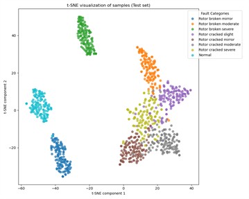
To better understand the performance with varying training sample sizes, we take the model with no prior training, the models trained on Datasets A1, A2, and A3, and plot the t-SNE visualization results of test samples to observe generalization on unseen data, as shown in Fig 5. We observe overall changes in the feature space: after training, samples of the same class cluster well, and with more training samples, classification boundaries become clearer.

Fig. 4The average accuracy (%) of 10 tests of different methods in few-shot diagnosis experiments

A more detailed analysis shows that, as seen in Fig. 5(a), the Normal class samples, Rotor broken mirror samples, and Rotor broken mirror samples achieve excellent clustering results with simple dimensionality reduction techniques, while the other classes show irregular distributions. In Fig. 5(b), when the training sample size is small, most of the test samples fit well, but the classification boundary for the Rotor broken moderate class and Rotor cracked fault classes is somewhat fuzzy. This may lead to misclassification of Rotor cracked faults. However, as shown in Fig. 5(c), as the number of labeled training samples increases, the classification boundaries for the Rotor cracked fault classes become clearer, reflecting that the MSCSN model gradually reduces the likelihood of misclassifying Rotor cracked faults. Overall, across various labeled training sample sizes and different support set sizes, the proposed intelligent diagnostic model maintains a diagnostic accuracy greater than 90.54 %, with an average accuracy exceeding 92.56 %. This fully demonstrates that the proposed MSCSN model is suitable for few-shot fault diagnosis tasks in UAVs.

5.2. Performance of the model on various transfer tasks

In real UAV fault diagnosis applications, especially when the UAV operates under new conditions, an important challenge arises: how to effectively classify fault types without rebuilding a new model. Re-training a model typically requires significant computational resources and data, which undoubtedly increases costs. Therefore, to verify the knowledge transfer ability of the existing model under new conditions, this study adopts an evaluation strategy: 20 samples from the source domain dataset are input into the MSCSN model for training, while a subset of labeled samples from the target domain dataset is selected as the validation set, with the number of validation samples being 10, 15, and 20. Additionally, 120 remaining samples from the target domain are selected as the test set. In total, 12 transfer tasks are formed.

The process is divided into 12 different experimental tasks, aiming to comprehensively assess the model's adaptability and robustness under unknown operating conditions. In the experiments presented in Section 5.1, it has been shown that the proposed method outperforms the baseline network and Zhang’s net, so further testing with these models is excluded in the following experiments. The average diagnostic accuracy of 10 tests of MSCSN under different transfer tasks is shown in Table 6.

Fig. 5Data distribution of test samples under different training states

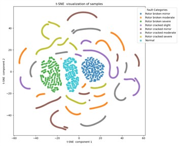
a) Before training

b) Dataset A1

c) Dataset A2

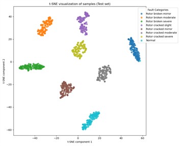
d) Dataset A3

From Table 6, it can be observed that the classification accuracy of each different domain transfer task varies significantly. Within the same transfer task category, as the number of training samples increases, the fault classification accuracy shows a corresponding upward trend. Further observation reveals that even when performing knowledge transfer between fixed domains, the selection of different source domains affects the final classification performance.

Table 6The average accuracy (%) of 10 tests with different domain transfer tasks

Task	Source domain	Target domain	Accuracy	Mean
1	Dataset A3	Dataset B1	92.28	93.81
2		Dataset B2	93.24
3		Dataset B3	95.91
4	Dataset B3	Dataset C1	85.01	91.15
5		Dataset C2	93.24
6		Dataset C3	95.21
7	Dataset B3	Dataset A1	91.12	92.62
8		Dataset A2	92.50
9		Dataset A3	94.23
10	Dataset C3	Dataset B1	84.43	90.28
11		Dataset B2	92.54
12		Dataset B3	93.87

Specifically, during the transfer between domains A and B, when using A as the source domain, the classification accuracy is, on average, 1.19 % higher than when using B as the source domain. Similarly, in the transfer between domains B and C, using B as the source domain results in a classification accuracy 0.87 % higher than using C as the source domain.

From the flight information presented in Table 3, it can be analyzed that Domain A, compared to Domain B, has smaller inertia characteristics and weaker vibration amplitude, making it more challenging to extract fault sample features from Domain A. In contrast, Domain B involves more complex flight tasks compared to Domain C, leading to more redundant information in fault sample features. This means that more samples are required to allow the model to learn accurate classification features effectively. Additionally, we believe that the performance decline from B to C, compared to A to B, may be due to larger signal differences in the former. The dynamic response time and system inertia during the ascent and descent process may have been relatively consistent in the A and B datasets, but the C dataset, due to stable hovering, may not have involved rapid changes and responses in system inertia.

The fine-tuning of MSCSN under different target domain training sample sizes, including the loss change over epochs for each transfer task, is shown in Fig. 6. It can be observed that, regardless of the target domain training sample size, the loss stabilizes after the first 10 epochs during the fine-tuning process. This is because the knowledge learned from the source domain training samples can be quickly transferred to the target domain. A detailed analysis and in-depth study of the experimental data reveal that UAVs, under diverse operating conditions, inevitably produce fault sample features with significant differences due to various factors such as flight posture and payload weight. Even under conditions with significant domain differences, the model maintains an accuracy of 84.43 %, fully demonstrating its stability and reliability under standard operating conditions.

Fig. 6The loss changes over epochs for each transfer task

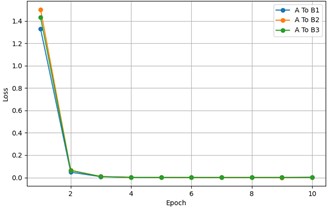
a) A To B

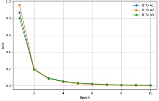
b) B To A

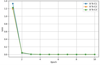
c) B To C

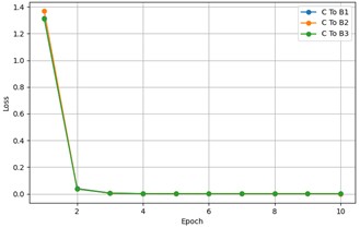
d) C To B

5.3. Performance of the model on the MVS-UAV-BF dataset

To further verify the general applicability of the proposed method, this study conducted validation using the MVS-UAV-BF dataset [38]. The test setup of this dataset which includes a multirotor UAV, an accelerometer sensor, healthy, damaged blades, and data acquisition. The experiment designed five fault states, each of which was independently applied to a single blade. For reference, the blade numbering follows a clockwise pattern when observed from top to bottom. The fault specific fault details listed in Table 7. The experimental environment is an indoor, fixed-height flight without wind. Each fault was recorded for 7 minutes of continuous acceleration vibration signals at a sampling frequency of 1024 Hz. Data were captured along the $X$ , $Y$ , and $Z$ axes, with approximately 400,000 data points per axis. The first 30 % of the data for each state was selected as the training set, and the remaining 70 % as the test set. Each data collection consisted of 2048 data points, with a sliding window moving 256 data points backward after each collection. A total of 50 training samples and 120 test samples were obtained.

Table 7The information for each fault type in the MVS-UAV-BF dataset

Fault type	Label	Fault location	Fault configuration
Healthy	Healthy	–	–
Mass removal fault	Unbalanced bottom right blade	Blade1	Sticky tape
Mass removal fault	Unbalanced top right blade	Blade2	Sticky tape
Weight unbalance fault	Damaged bottom right blade	Blade1	Shear
Weight unbalance fault	Damaged top right blade	Blade2	Shear

To explore the specific impact of the number of training samples on the performance of the Siamese network model, three dataset configurations, similar to those in Table 5, were set, and named Dataset 1, 2, and 3. The comparison of MSCSN model performance under three different training sample sizes is shown in Fig. 7, which demonstrates that the training sample size significantly affects the model’s convergence speed. As the total number of samples decreases, the model receives less information, resulting in a slower convergence and a longer training time. The accuracy improves more gradually. When a larger training sample size is used, the model reaches a low loss value after around 50 iterations, and the classification accuracy stabilizes above 91 %. Even with a smaller training sample size, after around 80 iterations, the loss value generally remains below 0.25, with the classification accuracy staying around 88 %. Ultimately, under all three sample configurations, stable classification accuracy was achieved. This highlights the excellent generalization capability of MSCSN when dealing with small sample problems.

5.4. Performance of the model on the ablation study

To observe the impact of hyperparameters on model performance, such as learning rate, batch size, and the boundary threshold in contrastive loss, we set three candidate values for each hyperparameter and conduct a sensitivity analysis to identify the optimal parameter combination. Additionally, in metric learning, common metric methods like cosine similarity and triplet loss will also be considered. Based on the optimal hyperparameters, we will compare the impact of different metric strategies on model performance.

5.4.1. Performance of the model on different hyperparameters

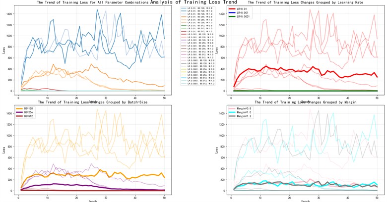
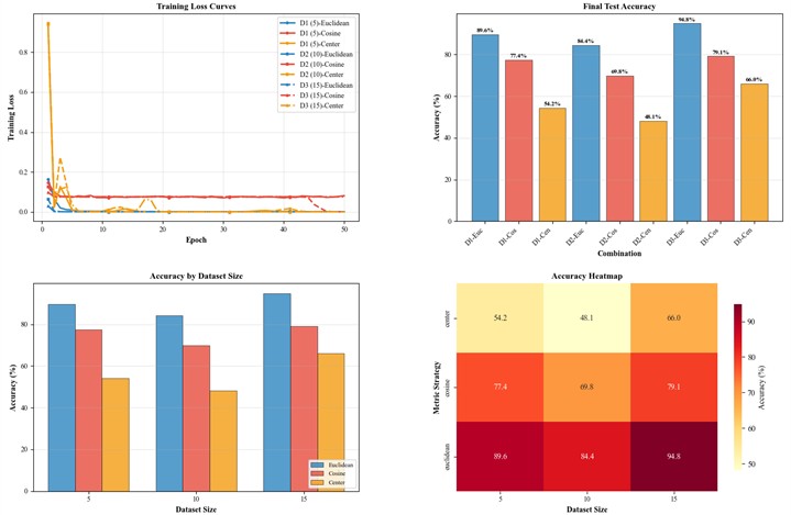
In this study, we aim to investigate the impact of three hyperparameters – Learning Rate, Batch Size, and Margin – on the performance of the proposed model. The learning rate is set to three possible values: 0.01, 0.001, and 0.0001; the batch size is set to three possible values: 128, 256, and 512; the margin in contrastive loss is set to three possible values: 0.8, 1.0, and 1.2, resulting in a total of 27 parameter combinations. We conducted 27 training sessions using Dataset A3, with each trained model tested three times. The experimental results are shown in Fig. 8. Additionally, we observed the change in training loss across different Epochs for the 27 parameter combinations, as shown in Fig. 9.

As can be seen from Fig. 8, the learning rate has a decisive impact on whether the model can effectively learn. When the learning rate is 0.01, the accuracy is only around 50 %. However, when the learning rate is 0.001, the model performs exceptionally well. At a learning rate of 0.0001, the accuracy remains between 80 % and 90 %. This is because, during backpropagation, a larger learning rate causes large updates to the learnable parameters, which may lead the model parameters to “skip” the optimal solution in the parameter space, resulting in fluctuating or unstable loss reduction. In contrast, a smaller learning rate results in more gradual updates to the parameters, allowing the model to fine-tune and converge to the optimal solution more precisely. We found that the best parameter combination for the highest accuracy is (0.001, 256, 1.0). However, when the margin is set to 1.2, the classification performance is generally more stable than when the margin is set to 1.0. Therefore, we chose 1.2 as the final margin value.

Fig. 7Network training performance with different sample sets

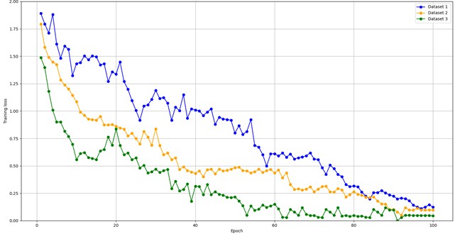
a) Loss curve

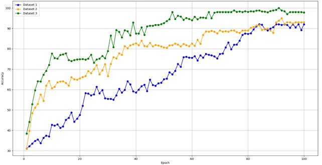
b) Accuracy curve

Fig. 9 includes four subplots, with the thick lines representing the average changes. The top-left subplot shows the trend of training loss across different parameter combinations. It can be seen that there is a significant difference in training loss between combinations. The top-right subplot shows the effect of different learning rates on training loss. With a learning rate of 0.01, the training loss fails to effectively converge. With a learning rate of 0.001, the loss curve is relatively stable and reaches a lower final loss. With a learning rate of 0.0001, the convergence is slower, but due to the larger number of iterations, the loss eventually converges. The loss values for the latter two are similar and small, which results in overlapping lines. In practical applications, a learning rate of 0.001 effectively reduces the number of iterations. This is because a larger learning rate causes the gradient updates to be too large, leading to missed optimal convergence paths, and may even prevent convergence. On the other hand, a smaller learning rate results in slower convergence and may require more epochs to achieve better performance, potentially getting stuck in local minima. The bottom-left subplot shows the change in training loss for different batch sizes. A batch size of 128 shows more significant fluctuations, with slower loss reduction in the early stages. For batch sizes of 256 and 512, the training loss stabilizes, gradually decreasing and leveling off. Notably, the setting of 256 performs best during the final convergence phase. This is because, while smaller batch sizes are computationally efficient, they are more susceptible to fluctuations caused by outliers. Larger batch sizes help achieve more accurate gradient estimation, allowing the model to converge more smoothly. The bottom-right subplot shows the effect of different margin thresholds on training loss, which has little impact on convergence. This indicates that the margin does not directly affect the training loss convergence process. In summary, learning rate and batch size significantly influence the model’s convergence speed, while selecting the appropriate margin is crucial for forming clear classification boundaries.

Fig. 8Performance of the model on different hyperparameters

Fig. 9The change in training loss across different Epochs for the 27 parameter combinations

5.4.2. Performance of the model on different metric strategies

We analyzed the adaptability of common metric strategies such as contrastive loss, cosine similarity loss, and center loss in the model proposed in this paper. Under the condition that the other modules remain unchanged, we selected the parameter combination (0.001, 256, 1.2), and retrained the model by changing the similarity metric using DatasetD1, DatasetD2, and DatasetD3. The results of the training are shown in Fig. 10. As can be seen from Fig. 10, the contrastive loss metric is more suitable for the model proposed in this paper compared to the other two strategies. Our analysis suggests that this is because contrastive loss directly measures the absolute distance between two samples in the feature space, making it effective in handling features with different magnitudes or units. For high-dimensional data such as vibration signals, the absolute distance between features often contains sufficient information to distinguish between samples of different categories. Therefore, using Euclidean distance in contrastive loss can more directly reflect the differences between samples, especially when dealing with features with varying magnitudes. In contrast, cosine similarity loss primarily measures the directional similarity between vectors, without considering the specific size or magnitude of the vectors. When dealing with vibration signals or similar data, this approach may overlook critical fault information. Center loss, on the other hand, mainly focuses on tightly clustering samples within the same category during optimization and does not directly impose constraints on the separation between categories. As a result, there may be overlap between categories, leading to poor classification performance, especially when there are many categories or when the samples are complex.

Fig. 10Performance of different metric strategies in MSCSN

6. Conclusions

This study proposes a UAV fault diagnosis method based on a multi-scale convolutional Siamese network. The method combines a Siamese network with an improved multi-scale convolutional network to automatically extract multi-level fault features. Using Euclidean distance-based metrics and contrastive loss, the model ensures that samples of the same class are compact in feature space, while the distance between samples from different classes is significantly larger, leading to better classification boundaries. Experimental results show that, across three training sample sizes, the model achieves an average diagnostic accuracy of no less than 90.54 %. In cross-domain transfer tasks, the method achieves an average accuracy of no less than 84.43 % in diverse flight environments. We also conducted sensitivity analysis of model parameters and an evaluation of various metric strategies for model adaptation. Additionally, experiments on the public dataset MVS-UAV-BF demonstrated that the proposed model exhibits stable generalization performance in small-sample UAV fault diagnosis.

The significant contribution of this study lies in proposing a potential UAV fault diagnosis solution. Given its performance in transfer tasks and on the public dataset, the model is shown to be suitable for a broad range of rotary-wing UAV fault diagnosis tasks. Although there is room for further improvement in accuracy, the lightweight nature of the model reduces the risk of overfitting in small-sample scenarios and shortens fault diagnosis time.

However, there are still limitations in our study, such as the need to verify the model's stability in more complex dynamic flight scenarios and its ability to detect subtle faults with fewer samples. These represent potential directions for future research.

References

S. G. Eladl, A. Y. Haikal, M. M. Saafan, and H. Y. Zaineldin, “A proposed plant classification framework for smart agricultural applications using UAV images and artificial intelligence techniques,” Alexandria Engineering Journal, Vol. 109, pp. 466–481, Dec. 2024, https://doi.org/10.1016/j.aej.2024.08.076

Publisher
H. Noh, S. Kwon, Y. S. Park, and S.-B. Woo, “Application of RGB UAV imagery to sea surface suspended sediment concentration monitoring in coastal construction site,” Applied Ocean Research, Vol. 145, p. 103940, Apr. 2024, https://doi.org/10.1016/j.apor.2024.103940

Publisher
C.-H. Huang, Y.-C. Chen, C.-Y. Hsu, J.-Y. Yang, and C.-H. Chang, “FPGA-based UAV and UGV for search and rescue applications: A case study,” Computers and Electrical Engineering, Vol. 119, p. 109491, Oct. 2024, https://doi.org/10.1016/j.compeleceng.2024.109491

Publisher
M. Castellani, M. A., G.-M. E., A. F., and U. F., “UAV photogrammetry and laser scanning of bridges: a new methodology and its application to a case study,” Procedia Structural Integrity, Vol. 62, pp. 193–200, Jan. 2024, https://doi.org/10.1016/j.prostr.2024.09.033

Publisher
Y. Chen, C. Zhang, Q. Zhang, and X. Hu, “UAV fault detection based on GA-BP neural network,” in 2017 32nd Youth Academic Annual Conference of Chinese Association of Automation (YAC), pp. 806–811, May 2017, https://doi.org/10.1109/yac.2017.7967520

Publisher
G. Iannace, G. Ciaburro, and A. Trematerra, “Fault diagnosis for UAV blades using artificial neural network,” Robotics, Vol. 8, No. 3, p. 59, Jul. 2019, https://doi.org/10.3390/robotics8030059

Publisher
X.-M. Chen et al., “Design and analysis for early warning of rotor UAV based on data-driven DBN,” Electronics, Vol. 8, No. 11, p. 1350, Nov. 2019, https://doi.org/10.3390/electronics8111350

Publisher
L. Yang et al., “An unmanned aerial vehicle troubleshooting mode selection method based on SIF-SVM with fault phenomena text record,” Aerospace, Vol. 8, No. 11, p. 347, Nov. 2021, https://doi.org/10.3390/aerospace8110347

Publisher
D. Guo, M. Zhong, H. Ji, Y. Liu, and R. Yang, “A hybrid feature model and deep learning based fault diagnosis for unmanned aerial vehicle sensors,” Neurocomputing, Vol. 319, pp. 155–163, Nov. 2018, https://doi.org/10.1016/j.neucom.2018.08.046

Publisher
J. Wang, J. Miao, J. Wang, F. Yang, K.-L. Tsui, and Q. Miao, “Fault diagnosis of electrohydraulic actuator based on multiple source signals: An experimental investigation,” Neurocomputing, Vol. 417, pp. 224–238, Dec. 2020, https://doi.org/10.1016/j.neucom.2020.05.102

Publisher
L. Wen, X. Li, L. Gao, and Y. Zhang, “A new convolutional neural network-based data-driven fault diagnosis method,” IEEE Transactions on Industrial Electronics, Vol. 65, No. 7, pp. 5990–5998, Jul. 2018, https://doi.org/10.1109/tie.2017.2774777

Publisher
N. Wang, J. Ren, Y. Luo, K. Guo, and D. Liu, “UAV actuator fault detection using maximal information coefficient and 1-d convolutional neural network,” in Global Reliability and Prognostics and Health Management (PHM-Nanjing), Oct. 2021, https://doi.org/10.1109/phm-nanjing52125.2021.9613071

Publisher
C. Du et al., “Unmanned aerial vehicle rotor fault diagnosis based on interval sampling reconstruction of vibration signals and a one-dimensional convolutional neural network deep learning method,” Measurement Science and Technology, Vol. 33, No. 6, p. 065003, Jun. 2022, https://doi.org/10.1088/1361-6501/ac491e

Publisher
K. Guo, N. Wang, D. Liu, and X. Peng, “Uncertainty-aware LSTM based dynamic flight fault detection for UAV actuator,” IEEE Transactions on Instrumentation and Measurement, Vol. 72, pp. 1–13, Jan. 2023, https://doi.org/10.1109/tim.2022.3225040

Publisher
W. Luo, H. Ebel, and P. Eberhard, “An LSTM‐based approach to precise landing of a UAV on a moving platform,” International Journal of Mechanical System Dynamics, Vol. 2, No. 1, pp. 99–107, Apr. 2022, https://doi.org/10.1002/msd2.12036

Publisher
G. Chen et al., “Fault diagnosis of drone motors driven by current signal data with few samples,” Measurement Science and Technology, Vol. 35, No. 8, p. 086202, Aug. 2024, https://doi.org/10.1088/1361-6501/ad3d00

Publisher
Q. Hang, J. Yang, and L. Xing, “Diagnosis of rolling bearing based on classification for high dimensional unbalanced data,” IEEE Access, Vol. 7, pp. 79159–79172, Jan. 2019, https://doi.org/10.1109/access.2019.2919406

Publisher
L. Duan, M. Xie, T. Bai, and J. Wang, “A new support vector data description method for machinery fault diagnosis with unbalanced datasets,” Expert Systems with Applications, Vol. 64, pp. 239–246, Dec. 2016, https://doi.org/10.1016/j.eswa.2016.07.039

Publisher
J. Yang, X. Guo, Y. Li, F. Marinello, S. Ercisli, and Z. Zhang, “A survey of few-shot learning in smart agriculture: developments, applications, and challenges,” Plant Methods, Vol. 18, No. 1, p. 28, Mar. 2022, https://doi.org/10.1186/s13007-022-00866-2

Publisher
Y. Liu, H. Zhang, W. Zhang, G. Lu, Q. Tian, and N. Ling, “Few-shot image classification: current status and research trends,” Electronics, Vol. 11, No. 11, p. 1752, May 2022, https://doi.org/10.3390/electronics11111752

Publisher
R. Zhang and Q. Liu, “Learning with few samples in deep learning for image classification, a mini-review,” Frontiers in Computational Neuroscience, Vol. 16, p. 10752, Jan. 2023, https://doi.org/10.3389/fncom.2022.1075294

Publisher
S. Tian, L. Li, W. Li, H. Ran, X. Ning, and P. Tiwari, “A survey on few-shot class-incremental learning,” Neural Networks, Vol. 169, pp. 307–324, Jan. 2024, https://doi.org/10.1016/j.neunet.2023.10.039

Publisher
M. R. Bhuiyan and J. Uddin, “Deep transfer learning models for industrial fault diagnosis using vibration and acoustic sensors data: a review,” Vibration, Vol. 6, No. 1, pp. 218–238, Feb. 2023, https://doi.org/10.3390/vibration6010014

Publisher
T. Pan, J. Chen, T. Zhang, S. Liu, S. He, and H. Lv, “Generative adversarial network in mechanical fault diagnosis under small sample: A systematic review on applications and future perspectives,” ISA Transactions, Vol. 128, pp. 1–10, Sep. 2022, https://doi.org/10.1016/j.isatra.2021.11.040

Publisher
X. Liang, M. Zhang, G. Feng, D. Wang, Y. Xu, and F. Gu, “Few-shot learning approaches for fault diagnosis using vibration data: a comprehensive review,” Sustainability, Vol. 15, No. 20, p. 14975, Oct. 2023, https://doi.org/10.3390/su152014975

Publisher
Z. Xu, K. Zhao, J. Wang, and M. Bashir, “Physics-informed probabilistic deep network with interpretable mechanism for trustworthy mechanical fault diagnosis,” Advanced Engineering Informatics, Vol. 62, p. 102806, Oct. 2024, https://doi.org/10.1016/j.aei.2024.102806

Publisher
C. Lai, P. Baraldi, and E. Zio, “Physics-informed deep autoencoder for fault detection in new-design systems,” Mechanical Systems and Signal Processing, Vol. 215, p. 111420, Jun. 2024, https://doi.org/10.1016/j.ymssp.2024.111420

Publisher
M. Zarchi, M. Shahgholi, and K. F. Tee, “An adaptable physics-informed fault diagnosis approach via hybrid signal processing and transferable feature learning for structural/machinery health monitoring,” Signal, Image and Video Processing, Vol. 18, No. 12, pp. 9051–9066, Sep. 2024, https://doi.org/10.1007/s11760-024-03529-y

Publisher
Z. Xu, Z. Jia, Y. Wei, S. Zhang, Z. Jin, and W. Dong, “A strong anti-noise and easily deployable bearing fault diagnosis model based on time-frequency dual-channel Transformer,” Measurement, Vol. 236, p. 115054, Aug. 2024, https://doi.org/10.1016/j.measurement.2024.115054

Publisher
B. Yuan, L. Lu, and S. Chen, “Research on bearing fault diagnosis based on vibration signals and deep learning models,” Electronics, Vol. 14, No. 10, p. 2090, May 2025, https://doi.org/10.3390/electronics14102090

Publisher
L. Jiang, J. Chen, H. Cao, P. Li, and K. Wang, “A novel bearing fault diagnosis method using a hybrid TCN-transformer architecture: A deep learning approach,” Journal of Mechanical Science and Technology, Vol. 39, No. 7, pp. 3821–3834, Jul. 2025, https://doi.org/10.1007/s12206-025-0607-5

Publisher
X. Li, G. Zhu, A. Hu, L. Xing, and L. Xiang, “A meta-learning method based on meta-feature enhancement for bearing fault identification under few-sample conditions,” Mechanical Systems and Signal Processing, Vol. 226, p. 112370, Mar. 2025, https://doi.org/10.1016/j.ymssp.2025.112370

Publisher
J. Luo, H. Shao, J. Lin, and B. Liu, “Meta-learning with elastic prototypical network for fault transfer diagnosis of bearings under unstable speeds,” Reliability Engineering and System Safety, Vol. 245, p. 110001, May 2024, https://doi.org/10.1016/j.ress.2024.110001

Publisher
J. Tang et al., “A prior knowledge-enhanced self-supervised learning framework using time-frequency invariance for machinery intelligent fault diagnosis with small samples,” Engineering Applications of Artificial Intelligence, Vol. 133, p. 108503, Jul. 2024, https://doi.org/10.1016/j.engappai.2024.108503

Publisher
C. Pan, Z. Shang, L. Tang, H. Cheng, and W. Li, “Open-set domain adaptive fault diagnosis based on supervised contrastive learning and a complementary weighted dual adversarial network,” Mechanical Systems and Signal Processing, Vol. 222, p. 111780, Jan. 2025, https://doi.org/10.1016/j.ymssp.2024.111780

Publisher
A. Zhang, S. Li, Y. Cui, W. Yang, R. Dong, and J. Hu, “Limited data rolling bearing fault diagnosis with few-shot learning,” IEEE Access, Vol. 7, pp. 110895–110904, Jan. 2019, https://doi.org/10.1109/access.2019.2934233

Publisher
F. Jiang et al., “A novel dual attention convolutional neural network based on multisensory frequency features for unmanned aerial vehicle rotor fault diagnosis,” IEEE Access, Vol. 11, pp. 99950–99960, Jan. 2023, https://doi.org/10.1109/access.2023.3314193

Publisher
L. A. Al-Haddad, A. A. Jaber, M. N. Hamzah, H. Kraiem, M. I. Al-Karkhi, and A. Flah, “Multiaxial vibration data for blade fault diagnosis in multirotor unmanned aerial vehicles,” Scientific Data, Vol. 12, No. 1, p. 1383, Aug. 2025, https://doi.org/10.1038/s41597-025-05692-4

Publisher

About this article

Received

June 4, 2025

Accepted

November 3, 2025

Published

December 14, 2025

SUBJECTS

Fault diagnosis based on vibration signal analysis

DOI

https://doi.org/10.21595/jve.2025.25101

Keywords

UAV fault diagnosis

few-shot learning

multi-scale convolutional neural network (MSCNN)

Siamese network

metric learning

Acknowledgements

This research has been supported by the Guangdong Provincial Key Field Special Project (High and Equipment Manufacturing No. 2023ZDZX3009), and the Guangdong Basic and Applied Basic Research Foundation (Grant No. 2024A1515010166), and the Guangdong Association for Science and Technology Youth Science and Technology Talents Training Program (Grant No. SKXRC2025450).

Data Availability

The datasets generated during and/or analyzed during the current study are available from the corresponding author on reasonable request.

Author Contributions

Tubao Han: methodology, investigation, validation, writing-original draft preparation and writing-review and editing. Canyi Du: project administration, writing-review and editing. Xiaoqing Yang: supervision and resources. Yongxian Huang: supervision, conceptualization and methodology. Xiangkun Zeng: data curation and software. Feifei Yu: data curation and supervision. Yongkang Gong: investigation, data curation. Junyi Zhang: investigation, validation. Wenzhu Zhou: translating and editing. Jie Qi: data curation.

Conflict of interest

The authors declare that they have no conflict of interest.

This is an open access article distributed under the Creative Commons Attribution License, which permits unrestricted use, distribution, and reproduction in any medium, provided the original work is properly cited.

T. Han et al., “A multi-scale convolutional Siamese network for few-shot fault diagnosis of unmanned aerial vehicle rotor,” Journal of Vibroengineering, Vol. 27, No. 8, –19, Dec. 2025, https://doi.org/10.21595/jve.2025.25101

Copy Extrica

Copied to clipboard!

TY  - JOUR
DO  - 10.21595/jve.2025.25101
UR  - https://doi.org/10.21595/jve.2025.25101
TI  - A multi-scale convolutional Siamese network for few-shot fault diagnosis of unmanned aerial vehicle rotor
T2  - Journal of Vibroengineering
AU  - Han, Tubao
AU  - Du, Canyi
AU  - Yang, Xiaoqing
AU  - Huang, Yongxian
AU  - Zeng, Xiangkun
AU  - Yu, Feifei
AU  - Gong, Yongkang
AU  - Zhang, Junyi
AU  - Zhou, Wenzhu
AU  - Qi, Jie
PY  - 2025
DA  - 2025/12/14
PB  - Extrica
VL  - 27
IS  - 8
SN  - 1392-8716
SN  - 2538-8460
ER  - 

Copy Ris

Copied to clipboard!

 @article{Han_2025, title={A multi-scale convolutional Siamese network for few-shot fault diagnosis of unmanned aerial vehicle rotor}, ISSN={2538-8460}, url={https://doi.org/10.21595/jve.2025.25101}, DOI={10.21595/jve.2025.25101}, journal={Journal of Vibroengineering}, publisher={JVE International Ltd.}, author={Han, Tubao and Du, Canyi and Yang, Xiaoqing and Huang, Yongxian and Zeng, Xiangkun and Yu, Feifei and Gong, Yongkang and Zhang, Junyi and Zhou, Wenzhu and Qi, Jie}, year={2025}, month=dec }

Copy Bibtex

Copied to clipboard!

[1]T. Han et al., “A multi-scale convolutional Siamese network for few-shot fault diagnosis of unmanned aerial vehicle rotor,” Journal of Vibroengineering, Dec. 2025, doi: 10.21595/jve.2025.25101.

Copy IEEE

Copied to clipboard!

Han, Tubao, Canyi Du, Xiaoqing Yang, Yongxian Huang, Xiangkun Zeng, Feifei Yu, Yongkang Gong, Junyi Zhang, Wenzhu Zhou, and Jie Qi. “A Multi-Scale Convolutional Siamese Network for Few-Shot Fault Diagnosis of Unmanned Aerial Vehicle Rotor.” Journal of Vibroengineering, December 14, 2025. https://doi.org/10.21595/jve.2025.25101.

Copy Chicago

Copied to clipboard!

A multi-scale convolutional Siamese network for few-shot fault diagnosis of unmanned aerial vehicle rotor

Abstract

1. Introduction

2. Related work

3. Proposed method

3.1. Preprocessing module

3.2. Feature extraction module

3.3. Metric module

4. Rotor blade fault diagnosis dataset

5. Model validation

5.1. Performance of the model under different training sample sizes

5.2. Performance of the model on various transfer tasks

5.3. Performance of the model on the MVS-UAV-BF dataset

5.4. Performance of the model on the ablation study

5.4.1. Performance of the model on different hyperparameters

5.4.2. Performance of the model on different metric strategies

6. Conclusions

References

About this article

Related Articles