Abstract
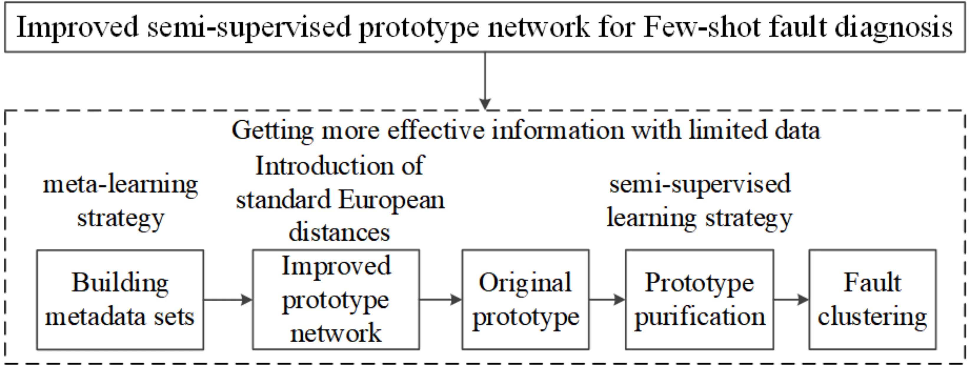
The collection of labeled data for transient mechanical faults is limited in practical engineering scenarios. However, the completeness of sample determines quality for feature information, which is extracted by deep learning network. Therefore, to obtain more effective information with limited data, this paper proposes an improved semi-supervised prototype network (ISSPN) that can be used for fault diagnosis. Firstly, a meta-learning strategy is used to divide the sample data. Then, a standard Euclidean distance metric is used to improve the SSPN, which maps the samples to the feature space and generates prototypes. Furthermore, the original prototypes are refined with the help of unlabeled data to produce better prototypes. Finally, the classifier clusters the various faults. The effectiveness of the proposed method is verified through experiments. The experimental results show that the proposed method can do a better job of classifying different faults.
Highlights
- The use of the standard Euclidean distance metric function eliminates the variability caused by different scales and improves the robustness of the model.
- A semi-supervised learning strategy is used to make full use of unlabelled data and obtain more accurate prototypes.
- Improved prototype network obtains more effective features with limited data and solves few-shot problems effectively
- Experiments verify that the method can accurately identify various types of faults with good generalisation performance under few-shot conditions.
1. Introduction
The complete sample of monitoring data is the foundation of fault diagnosis for mechanical equipment [1], [2]. However, the collected data is usually limited and constitutes few-shot instances for mechanical condition monitoring, thus making it difficult to identify fault information. Therefore, intelligent diagnosis methods are studied to address this problem [3-6]. Specially, deep learning (DL) shows excellent performance in solving small sample problems [7-10].
The fault diagnosis model based on deep learning could effectively identify fault features from few-shot data, therefore solving the problem of fault diagnosis under small sample condition. Saufi et al. [11] proposed a deep learning model based on stacked sparse autoencoders (SSAE) to tackle the small sample size problem. The experimental results show that the diagnosis model has high diagnosis performance. Ren et al. [12] designed a capsule autoencoder model (CaAE) for intelligent fault diagnosis. The state capsule has undergone feature fusion, which makes it easier to achieve better diagnosis accuracy with smaller training samples. In addition, with the help of relevant datasets, feature adaptation based on transfer learning can also learn fault features from few-shot datasets to achieve accurate fault diagnosis. Xie and Duan used transfer component analysis (TCA) to extract transferable fault features from gearbox vibration signals. These two models can effectively extract and fuse cross-domain features [13], [14]. However, it is not ideal in terms of the actual accuracy for transfer learning method due to the complex high-dimensional data and negative transfer.
Meta-learning can more effectively complete the classification of faults by virtue of its unique training methods and strong generalization ability, addressing the problem of insufficient samples. Yu et al. [15] designed a meta-learning model based on time-frequency features and multi-label convolutional neural networks. It can quickly identify new fault types by a few samples and a simple network update step. Wang et al. [16] proposed an improved metric meta-learning model. The approach makes full use of the attribute information of a single sample and the similarity information between sample groups. Chen et al. [17] have constructed an improved prototype network model with frequency domain data as input. The network uses Mahalanobis distance instead of Euclidean distance for prototype classification. Although the above meta-learning methods have achieved considerable results, they mainly focus on labeled samples and ignore the information existing in unlabeled samples.
In practical engineering, most of the collected data is unlabeled, leading to increased costs and time for labeling each sample individually. To address this issue, scholars have conducted further studies on semi-supervised learning due to its ability to generate stronger feature representations for each class [18-20]. Yu et al. [21] proposed an effective semi-supervised learning method based on the principle of consistent regularization, which could enhance the clustering between features through supervised and unsupervised loss terms. But this adds a large number of additional enhancement operations. Feng et al. [22] proposed a semi-supervised local Fisher discriminant network by adopting a pseudo-labeling strategy. It has an excellent performance for reducing the number of enhancement operations. Nevertheless, this network is more suitable for processing high-dimensional image data. This paper incorporates a semi-supervised learning strategy into the prototype network framework. The prototypes of all classes are refined multiple times by predicting the labels of unlabeled data to enhance the features of the individual prototypes [23-26].
In this paper, an improved semi-supervised prototype network (ISSPN) is designed to accomplish small sample fault classification with limited data. In this method, ProtoNet-based metric meta-learning network is used to extract fault features efficiently with limited data. Then, a semi-supervised learning strategy is employed, where unlabeled data is used to improve the quality of the prototypes for better fault clustering. Finally, the use of standard Euclidean distance instead of Euclidean distance in the prototype distance metric can eliminate the effect of differences in different feature scales. Meanwhile, the standardization of the data also reduces the impact of outliers on the distance calculation and improves the robustness of the model to outliers.
The rest of the paper is organized as follows: Section 2 outlines the relevant theory. Section 3 describes the proposed method and model in detail. Sections 4 and 5 are devoted to experimental analysis and conclusions, respectively.
2. Basic theory
2.1. Prototypical networks
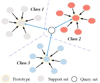
Prototypical Networks (ProtoNet) is a typical metric-based meta-learning model. This network maps the data into different classes by the feature function, and then learns the similarity between each sample by the distance metric [27], as illustrated in Fig. 1. Specifically, since ProtoNet operates on a meta-learning framework, it adheres to a scenario training strategy. Firstly, the dataset is divided into multiple tasks using the “N-way K-shot” approach. This means that each task comprises N classes, with each class containing K samples. Moreover, each task consists of a support set S (training set) and a query set Q (test set). The task is divided into two parts during the training process: the meta-training set and the meta-test set. Simultaneously, the types of data in the two are different [28].
Next, the training process can be more accurately described as that the prototype network mainly learns a nonlinear feature mapping function . It is parameterized as a neural network to map the prototype into a feature space. In this space, prototypes from the same class are closer, while prototypes from different classes are far away from each other. All parameters of prototype networks depend on the feature mapping function. To calculate the prototype of each class , the average value of the mapped feature vector represents the prototype. The calculation is as follows:
where is the prototype of class , represents the total size of samples in class , is the sample belonging to class and is the label corresponding to .
Finally, the parameter e of the feature function is trained and updated by the query set samples under each meta-task. The classification of the sample is done by measuring the distance between the sample and all prototypes. The prediction probability of the sample belonging to the query set of class d is calculated as follows:
For the prototype of all query sets, the loss function is defined to update the average negative logarithm of all query set samples in a given training set:
where is the total number of samples in the query set . The training process updates the model parameters by minimizing .
Fig. 1Schematic representation of a metric-based meta-learning model
2.2. Prototype purification
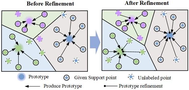
Due to the small amount of sample data and the limited number of labeled samples, the initial prototype cannot correctly represent the cluster centroid. To get a better prototype, the unlabeled data is used to adjust the initial prototype. It can effectively solve the problem of position deviation caused by the limited labeled support data. The prototype can be guided slightly by the unlabeled samples, thereby better aggregating the information into the initial prototype. The prototype purification process is shown in Fig. 2.
First, the unlabeled data is assigned probability labels. And then, the probabilities of unlabeled data are aggregated into the existing prototypes to obtain more information. The initial prototype is constructed for each class with the labeled support set as shown in Eq. (1). Therefore, the probability of labeling the sample for each class can be given as follows:
The is a dataset that supports centralized labeling. The unlabeled data probability is shown in Eq. (5):
Fig. 2Schematic diagram of prototype purification
The standard Euclidean distance function is defined as:
where ; is the standard deviation corresponding to the prototype. For the refined prototype, two probability weight coefficients are defined as:
Whereupon the original prototype is assigned by weight coefficient corresponding to each category:
The and are the number of labeled and unlabeled samples in the support set, respectively.
At last, the process of refining the prototype is completed by repeatedly executing the Eq. (9) and continuously assigning the value of to .
3. The proposed method
In this section, the improved semi-supervised prototype network (ISSPN) is described in three parts. The approach is based on an extension of metric meta-learning. In the first part, the learning style of the method is introduced. Next, the process of diagnosis is described in detail. Finally, the optimizer is explained.
3.1. Learning style
The proposed method follows the way of semi-supervised few-shot learning in this paper. Foremost, the support set is divided into two parts: labeled sample and unlabeled sample :
After that, the labeled samples are then randomly selected for “N-way K-shot” classification. The labeled samples after classification are input into the model to obtain the initial prototypes of n categories. Moreover, samples in the unlabeled support set are input into the convolution operation blocks (COBs) module for mapping into the feature space. The unlabeled samples are used to adjust the position of initial prototype through multiple iterations until full convergence. In addition, part of the remaining samples are extracted from the classes as a query set , and then classify the samples in the query set by prototype purification. The prediction formula for each sample in the query set is given by:
where, indicates the probability of a sample in the query set belonging to class . Eventually, the model parameters are updated by calculating the loss of the model, and then back-propagated.
3.2. The diagnosis process of the proposed method
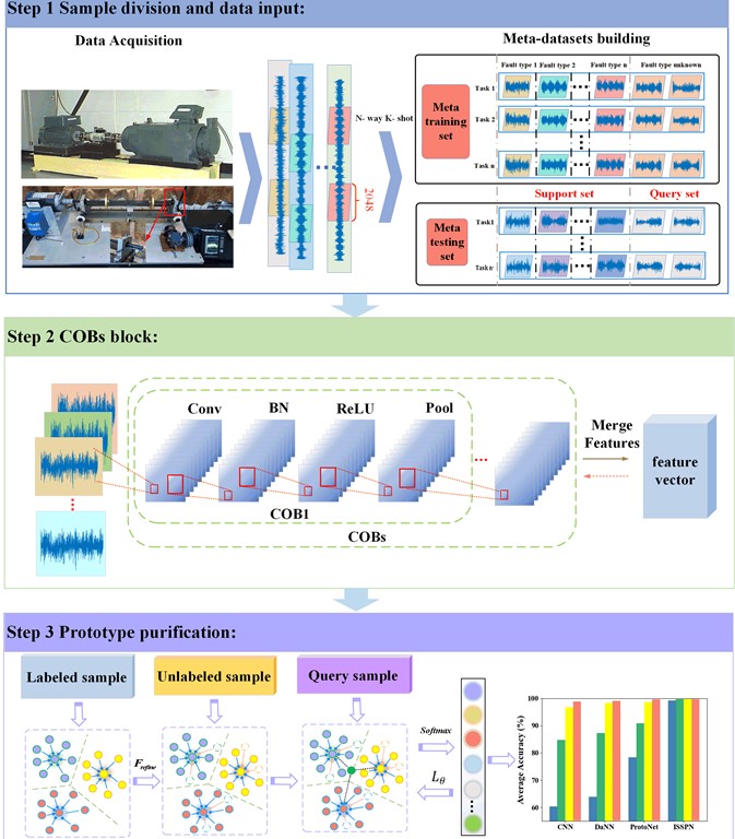
The general framework of the proposed method in this paper is shown in Fig. 3. The training process of method can be divided into four steps.
Step 1. Sample division and data input: The vibration acceleration signals of the bearing under different health conditions are collected. The meta-training set and the meta-test set contain multiple sets of 2048 data points generated by the time series signal, i.e., . According to the learning method proposed in Section 3.1, the sample can be represented as . Where is a labeled sample in the support set , is an unlabeled sample in the support set , and is the sample in the query set.
Step 2. COBs block: The data is mapped to a feature space and then merge all the channel features to obtain a mapped feature vector of . Therefore, A convolution operation block (COBs) consisting of multiple cobs of the same type is constructed, which include convolution block, batch normalization block, activation function ReLU and pooling layer. Consequently, a COBs block is designed to facilitate feature extraction. The module is capable of mapping input data to a feature space. The details about the convolutional operation block can be seen in Table 1. The flow chart of the structure is shown in the upper right block diagram in Fig. 3.
Specifically, a convolution operation is performed on the input data and the convolution kernel, thereby extracting the local input feature by sliding. The acceleration of the entire training process is achieved through the use of a batch normalization module. This approach also reduces the shift or disappearance of internal covariance, thus avoiding gradient explosion [29]. The input of th BN layer can be set , and the minibatch size is , so . The BN operation can be shown as follows:
where is BN layer output of the convolution result of the nth layer. and are the mean and variance of respectively. Usually, is a very small constant to prevent invalid calculations when the variance is zero, and the value is usually 1×10⁻⁵. Here, the parameters and are respectively the scale parameter and the offset parameter to be learned. They are initially set to 1 and 0, respectively.
Fig. 3ISSPN overall structure diagram
To make the features learned by the convolution layer easier to distinguish, the activation function becomes an indispensable part after convolution operation. The ReLU function is a frequently used to activation function in deep neural networks. It can enhance the sparsity of network. Its left saturation function alleviates the gradient vanishing problem of the neural network to a certain extent and accelerates the convergence speed of gradient descent. The ReLU is actually a ramp function, which is defined as follows:
where is the output of upper layer (BN layer), and is the activation amount of after activation by the ReLU function.
Further, the pooling layer is used to select features and reduce the dimension of features. The overfitting phenomenon can be effectively avoided by reducing the number of parameters. The maximum pooling operation can better complete the current task, and it can complete the local maximum operation on the input feature map.
To sum up, set and to be the dimension and length of the channel, respectively. The output of th convolution is . Therefore, the above COBs can be described as:
Finally, all the channel features are combined. The input data is also mapped to the feature space. Therefore, it can be described as:
where , is a -dimensional eigenvector. The input data also completes the feature mapping process by the COBs block, so the result is .
Step 3 Prototype Purification: The process of refining the prototype is completed by repeatedly executing the Eq. (9) and continuously assigning the value of to .To summarize, it can be generated the original prototype from the output obtained in the previous step. Meanwhile, the unlabeled data is assigned a predictable label . Furthermore, it is aggregated into the original prototype to guide the original prototype with deviation for adjusting the position in multiple iterations until convergence, so as to purify the prototype.
Table 1Details of the four methods
Block | Layer | Details |
COB | 1D-conv | 64 @ 1×3 |
BN | – | |
Activation | ReLU | |
1D-MaxPooling | 1×2 |
Step 4. Update the model: The sample in the query set is purified by the prototype to obtain its prediction probability and realize classification all at once. Furthermore, the model parameters are updated by calculating the loss of and propagating backward.
Although the stochastic gradient descent (SGD) optimizer can quickly reduce the loss in the early stage of training, it often struggles to converge to an optimal minimum value for the model loss. The ISSPN is trained more efficiently by using adaptive moment estimation, which computes bias-corrected first and second moment estimates to counteract bias. Moreover, it automatically adjusts the learning rate scale for different layers, eliminating the need for manual selection as in the case of SGD. Hence, it is easier to use [30].
4. Experimental analysis: The SQV bearing dataset
The performance of the proposed method is demonstrated by the collected bearing vibration dataset from a comprehensive mechanical failure test bed [31]. In order to fully prove the superiority of the method, three other methods are set up for comparison.
The first comparative experiment is set up on CNN whose feature extraction structure is consistent with the method in this paper. Similarly, DANN [32] can also be used as a good comparison object, which has the same feature extractor structure as ISSPN. DaNN is a CNN-based domain-adaptive deep neural network. It adjusts the difference between two domains by minimizing the Maximum Mean Difference (MMD) in the source domain and the target domain. The last group of comparative experiments is set in ProtoNet, which is the basis of this paper. Table 2 gives the details of the four methods including the proposed one in this paper. In addition, the results are characterized by visualization of tables, graphs, confusion matrices, and t-distributed random neighborhood embedding (t-SNE) [33].
Table 2Details of the four methods
Models | Learning style | Structure | Optimizer | |
Block | Classifier | |||
CNN | Supervised | 4*COB | Linear, Softmax | Adam |
DANN | Semi-Supervised | 4*COB | Linear, Softmax | Adam |
ProtoNet | Supervised FSL | 4*COB | Metric function | Adam |
ISSPN | Semi-Supervised FSL | 4*COB | Metric function | Adam |
4.1. Description of the dataset
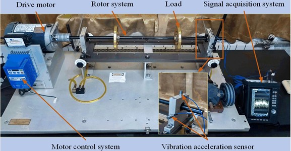
Due the fault signal characteristics of CWRU data set are very obvious. The validity of NSSPN method is further verified by collecting the bearing vibration signals of the comprehensive mechanical fault simulation test bench of the Spectral Mission (SQ) Company. Fig. 4 shows the integrated mechanical failure simulation test rig. The main part of the test bench is composed of driving motor, rotor system, motor control system, load and signal acquisition system. In the experiment, the vibration acceleration sensor is used to collect the bearing signal of the motor. The data acquisition instrument used is CoCo80, and the sampling frequency is 25.6 kHz. The experimental bearing is installed at the end of the drive motor, then a single point of failure is manually set on the experimental bearing. Specific information on the SQV bearing dataset is shown in Table 3. In addition, the experimental rotor system has four rotation frequencies (9 Hz, 19 Hz, 29 Hz, and 39 Hz). Fig. 5 shows a Time-Domain signal of the operating condition of the bearing at a rotation frequency of 39 Hz.
Fig. 4SQV bearing dataset test bench
4.2. Experimental parameter setting
To further evaluate the performance of the proposed method, two experiments are conducted on the SQV bearing dataset. The first experiment is three fault identifications (NC, IF-3 and OF-3) at four different speeds. First of all, a training data set is constructed: 100 samples are generated for each of the three fault conditions at each speed. So a total of 100×4×3 samples are generated. One to four samples are selected for each fault at each speed, resulting in four to sixteen samples for each type of fault. The number of unlabeled samples for ISSPN follows the support set, i.e. {1, 5} for each class. Ultimately, a single experiment and five experiments are set up to demonstrate the performance of the method, where each experiment is conducted for 30 iterations.
The second experiment is the identification of seven faults at one speed (39 Hz). Again, a data set needs to be constructed: 200 samples are generated for the 7 bearing States at 39 Hz, so a total of 1400 samples are generated. 5, 10, 20 and 30 samples are selected for each fault type. The training parameters are consistent with the above settings.
Fig. 5Time-domain signal of seven kinds of bearing vibration signals: a) mild inner ring fault (IF-1), b) moderate inner ring fault (IF-2), c) severe inner ring fault (IF-3), d) mild outer ring fault (OF-1), e) moderate outer ring fault (OF-2), f) severe outer ring fault (OF-3), g) normal condition (NC)
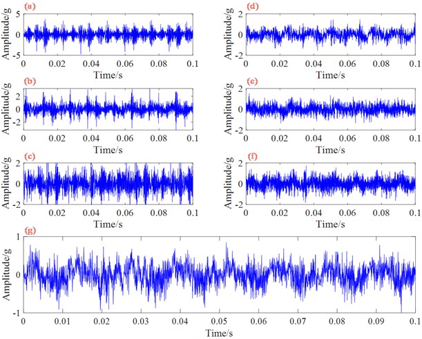
Table 3Details of SQV bearing dataset
Bearing condition | Fault damage degree | Damage scale (area/depth) |
Normal condition (NC) | Mild fault (1) | 4/0.5 |
Inner ring fault (IF) | Moderate fault (2) | 8/4 |
Outer ring fault (OF) | Severe Fault (3) | 12/2 |
4.3. Experimental results and analysis
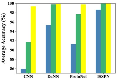
Table 4 shows the results of the three types of fault identification accuracy, and Fig. 6. visually shows the identification accuracy of each method. From the above tables and figures, it can be seen that although the accuracy of CNN, DaNN and ProtoNet is not less than 85 %, the ISSPN method shows better performance. The fault recognition rate of ISSPN can still reach 98.64 % when there are only 4 samples in each class. To sum up, the ISSPN method can adapt to fault diagnosis at different speeds by comparing with the other three methods.
Table 4Identification accuracy (%) of 3 types of faults on SQV dataset
Models | One experiment | Five experiments | ||||
4 | 10 | 16 | 4 | 10 | 16 | |
CNN | 85.94 | 91.67 | 99.38 | 90.75 | 99.05 | 100 |
DaNN | 95.32 | 99.78 | 99.86 | 96.74 | 99.85 | 100 |
ProtoNet | 91.27 | 97.69 | 99.79 | 97.19 | 100 | 100 |
ISSPN | 98.64 | 100 | 100 | 100 | 100 | 100 |
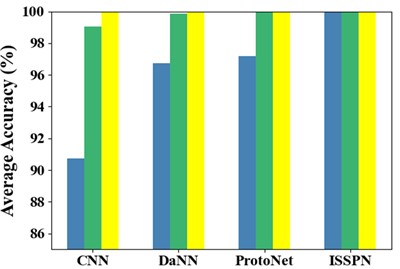
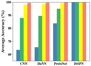
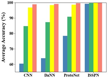
Besides, the accuracy results for the seven types of faults are shown in Table 5 and Fig. 7. The ISSPN method also shows excellent performance in the identification of seven types of faults by comparing with the other three methods. Similarly, the fault identification of ISSPN is still excellent when there are the fewest fault samples of each type. So it can be seen that the ISSPN method can complete the multi-class fault diagnosis excellently.
Fig. 6Accuracy of identification of three types of faults on SQV dataset: a) one experiment, b) five experiment
a)
b)
Table 5Identification accuracy (%) of 7 types of faults on SQV dataset
Models | One experiment | Five experiments | ||||||
5 | 10 | 20 | 30 | 5 | 10 | 20 | 30 | |
CNN | 60.38 | 84.76 | 96.78 | 98.89 | 63.46 | 87.94 | 98.04 | 99.43 |
DANN | 63.92 | 87.26 | 98.34 | 99.08 | 65.52 | 89.5 | 98.54 | 99.63 |
ProtoNet | 78.43 | 90.76 | 98.65 | 99.57 | 83.76 | 94.91 | 99.16 | 99.8 |
ISSPN | 99.27 | 99.73 | 100 | 100 | 99.86 | 99.94 | 100 | 100 |
Fig. 7Accuracy of identification of 7 types of faults on SQV dataset: a) one experiment, b) five experiment
a)
b)
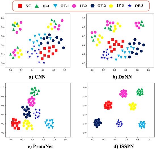
Taking the classification of seven types of faults as an example, Fig. 8 and Fig. 9 show the classification characterization results of ISSPN method in the form of confusion matrix and t-SNE visualization, respectively. It can be seen from the confusion matrix that the ISSPN method can accurately complete the classification of seven types of faults. The classification results of ISSPN method are also more obvious in the t-SNE visualization map. In summary, the ISSPN method has better feature extraction ability.
Fig. 8Confusion matrix of ISSPN seven-class classification results on SQV dataset
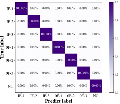
Fig. 9Visualization of t-SNE for the four methods on SQV dataset
5. Conclusions
This paper presents an improved semi-supervised learning network (ISSPN) for few-shot fault diagnosis. It can obtain more effective features with limited data, thus effectively solving the shot less problem in machinery fault diagnosis. The method adopts a semi-supervised learning strategy to make full use of unlabeled data to obtain more accurate prototypes. Meanwhile, the variability due to different scales is eliminated by the standard Euclidean distance metric function, which improves the robustness of the model. The performance of the method is validated with one case, and results show that the method can accurately identify all kinds of faults under the condition of few-shot and have good generalization performance. In addition, the performance of ISSPN is better compared to other similar methods.
References
-
Y. Lei, B. Yang, X. Jiang, F. Jia, N. Li, and A. K. Nandi, “Applications of machine learning to machine fault diagnosis: A review and roadmap,” Mechanical Systems and Signal Processing, Vol. 138, p. 106587, Apr. 2020, https://doi.org/10.1016/j.ymssp.2019.106587
-
D. Zhang, K. Zheng, Y. Bai, D. Yao, D. Yang, and S. Wang, “Few-shot bearing fault diagnosis based on meta-learning with discriminant space optimization,” Measurement Science and Technology, Vol. 33, No. 11, p. 115024, Nov. 2022, https://doi.org/10.1088/1361-6501/ac8303
-
Q. Wang, C. Yang, H. Wan, D. Deng, and A. K. Nandi, “Bearing fault diagnosis based on optimized variational mode decomposition and 1D convolutional neural networks,” Measurement Science and Technology, Vol. 32, No. 10, p. 104007, Oct. 2021, https://doi.org/10.1088/1361-6501/ac0034
-
Y. Wang and L. Cheng, “A combination of residual and long-short-term memory networks for bearing fault diagnosis based on time-series model analysis,” Measurement Science and Technology, Vol. 32, No. 1, p. 015904, Jan. 2021, https://doi.org/10.1088/1361-6501/abaa1e
-
Z. An, S. Li, J. Wang, and X. Jiang, “A novel bearing intelligent fault diagnosis framework under time-varying working conditions using recurrent neural network,” ISA Transactions, Vol. 100, pp. 155–170, May 2020, https://doi.org/10.1016/j.isatra.2019.11.010
-
S. Gao, L. Xu, Y. Zhang, and Z. Pei, “Rolling bearing fault diagnosis based on intelligent optimized self-adaptive deep belief network,” Measurement Science and Technology, Vol. 31, No. 5, p. 055009, May 2020, https://doi.org/10.1088/1361-6501/ab50f0
-
P. Peng, W. Zhang, Y. Zhang, Y. Xu, H. Wang, and H. Zhang, “Cost sensitive active learning using bidirectional gated recurrent neural networks for imbalanced fault diagnosis,” Neurocomputing, Vol. 407, pp. 232–245, Sep. 2020, https://doi.org/10.1016/j.neucom.2020.04.075
-
C. Zhang, K. C. Tan, H. Li, and G. S. Hong, “A cost-sensitive deep belief network for imbalanced classification,” IEEE Transactions on Neural Networks and Learning Systems, Vol. 30, No. 1, pp. 109–122, Jan. 2019, https://doi.org/10.1109/tnnls.2018.2832648
-
X. Li, H. Jiang, K. Zhao, and R. Wang, “A deep transfer nonnegativity-constraint sparse autoencoder for rolling bearing fault diagnosis with few labeled data,” IEEE Access, Vol. 7, No. 99, pp. 91216–91224, Jan. 2019, https://doi.org/10.1109/access.2019.2926234
-
Z. He, H. Shao, X. Zhang, J. Cheng, and Y. Yang, “Improved deep transfer auto-encoder for fault diagnosis of gearbox under variable working conditions with small training samples,” IEEE Access, Vol. 7, No. 99, pp. 115368–115377, Jan. 2019, https://doi.org/10.1109/access.2019.2936243
-
S. R. Saufi, Z. A. B. Ahmad, M. S. Leong, and M. H. Lim, “Gearbox fault diagnosis using a deep learning model with limited data sample,” IEEE Transactions on Industrial Informatics, Vol. 16, No. 10, pp. 6263–6271, Oct. 2020, https://doi.org/10.1109/tii.2020.2967822
-
Z. Ren et al., “A novel model with the ability of few-shot learning and quick updating for intelligent fault diagnosis,” Mechanical Systems and Signal Processing, Vol. 138, p. 106608, Apr. 2020, https://doi.org/10.1016/j.ymssp.2019.106608
-
L. Duan, J. Xie, K. Wang, and J. Wang, “Gearbox diagnosis based on auxiliary monitoring datasets of different working conditions,” Journal of Vibration and Shock, Vol. 36, No. 10, pp. 104–108, 2017, https://doi.org/10.13465/j.cnki.jvs.2017.10.017
-
J. Xie, L. Zhang, L. Duan, and J. Wang, “On cross-domain feature fusion in gearbox fault diagnosis under various operating conditions based on Transfer Component Analysis,” in 2016 IEEE International Conference on Prognostics and Health Management (ICPHM), Jun. 2016, https://doi.org/10.1109/icphm.2016.7542845
-
C. Yu, Y. Ning, Y. Qin, W. Su, and X. Zhao, “Multi-label fault diagnosis of rolling bearing based on meta-learning,” Neural Computing and Applications, Vol. 33, No. 10, pp. 5393–5407, Sep. 2020, https://doi.org/10.1007/s00521-020-05345-0
-
D. Wang, M. Zhang, Y. Xu, W. Lu, J. Yang, and T. Zhang, “Metric-based meta-learning model for few-shot fault diagnosis under multiple limited data conditions,” Mechanical Systems and Signal Processing, Vol. 155, No. 7, p. 107510, Jun. 2021, https://doi.org/10.1016/j.ymssp.2020.107510
-
Y. Chen, Y. Hong, J. Long, Z. Yang, Y. Huang, and C. Li, “Few shot learning for novel fault diagnosis with a improved prototypical network,” in 2021 International Conference on Sensing, Measurement and Data Analytics in the era of Artificial Intelligence (ICSMD), pp. 1–6, Oct. 2021, https://doi.org/10.1109/icsmd53520.2021.9670843
-
J. Kim, T. Kim, S. Kim, and C. D. Yoo, “Edge-labeling graph neural network for few-shot learning,” in 2019 IEEE/CVF Conference on Computer Vision and Pattern Recognition (CVPR), Jun. 2019, https://doi.org/10.1109/cvpr.2019.00010
-
X. Li et al., “Learning to self-train for semi-supervised few-shot classification,” arXiv:1906.00562, Jan. 2019, https://doi.org/10.48550/arxiv.1906.00562
-
Z. Yu, L. Chen, Z. Cheng, and J. Luo, “TransMatch: a transfer-learning scheme for semi-supervised few-shot learning,” in 2020 IEEE/CVF Conference on Computer Vision and Pattern Recognition (CVPR), Jun. 2020, https://doi.org/10.1109/cvpr42600.2020.01287
-
K. Yu, H. Ma, T. R. Lin, and X. Li, “A consistency regularization based semi-supervised learning approach for intelligent fault diagnosis of rolling bearing,” Measurement, Vol. 165, p. 107987, Dec. 2020, https://doi.org/10.1016/j.measurement.2020.107987
-
R. Feng, H. Ji, Z. Zhu, and L. Wang, “SelfNet: A semi-supervised local Fisher discriminant network for few-shot learning,” Neurocomputing, Vol. 512, pp. 352–362, Nov. 2022, https://doi.org/10.1016/j.neucom.2022.09.012
-
M. Ren et al., “Meta-learning for semi-supervised few-shot classification,” arXiv:1803.00676, Jan. 2018, https://doi.org/10.48550/arxiv.1803.00676
-
R. Boney and A. Ilin, “Semi-supervised and active few-shot learning with prototypical networks,” arXiv:1711.10856, Jan. 2017, https://doi.org/10.48550/arxiv.1711.10856
-
S. Basu and A. Banerjee, “Semi-supervised clustering by seeding,” in 19th International Conference on Machine Learning (ICML-2002), 2002, https://doi.org/10.5555/645531.656012
-
Y. Feng, J. Chen, T. Zhang, S. He, E. Xu, and Z. Zhou, “Semi-supervised meta-learning networks with squeeze-and-excitation attention for few-shot fault diagnosis,” ISA Transactions, Vol. 120, pp. 383–401, Jan. 2022, https://doi.org/10.1016/j.isatra.2021.03.013
-
Z. Ji, X. Chai, Y. Yu, Y. Pang, and Z. Zhang, “Improved prototypical networks for few-shot learning,” Pattern Recognition Letters, Vol. 140, pp. 81–87, Dec. 2020, https://doi.org/10.1016/j.patrec.2020.07.015
-
T. M. Hospedales, A. Antoniou, P. Micaelli, and A. J. Storkey, “Meta-learning in neural networks: a survey,” IEEE Transactions on Pattern Analysis and Machine Intelligence, pp. 1–1, Jan. 2021, https://doi.org/10.1109/tpami.2021.3079209
-
S. Ioffe and C. Szegedy, “Batch normalization: accelerating deep network training by reducing internal covariate shift,” arXiv:1502.03167, Jan. 2015, https://doi.org/10.48550/arxiv.1502.03167
-
D. P. Kingma and J. Ba, “Adam: a method for stochastic optimization,” arXiv:1412.6980, Jan. 2014, https://doi.org/10.48550/arxiv.1412.6980
-
Z. Shi, J. Chen, Y. Zi, and Z. Zhou, “A novel multitask adversarial network via redundant lifting for multicomponent intelligent fault detection under sharp speed variation,” IEEE Transactions on Instrumentation and Measurement, Vol. 70, No. 99, pp. 1–10, Jan. 2021, https://doi.org/10.1109/tim.2021.3055821
-
W. Lu, B. Liang, Y. Cheng, D. Meng, J. Yang, and T. Zhang, “Deep model based domain adaptation for fault diagnosis,” IEEE Transactions on Industrial Electronics, Vol. 64, No. 3, pp. 2296–2305, Mar. 2017, https://doi.org/10.1109/tie.2016.2627020
-
Laurens van der Maaten and Geoffrey Hinton, “Visualizing data using t-SNE,” Journal of Machine Learning Research, Vol. 9, No. 86, pp. 2579–2605, 2008.
About this article

The authors have not disclosed any funding.
The datasets generated during and/or analyzed during the current study are available from the corresponding author on reasonable request.
Zhenlian Lu: writing-review and editing, writing-original draft, validation, software, methodology, conceptualization. Kuosheng Jiang: writing-review and editing, validation, investigation, resources, funding acquisition. Jie Wu: writing-review and editing, validation, supervision, investigation, formal analysis.
The authors declare that they have no conflict of interest.
