Abstract
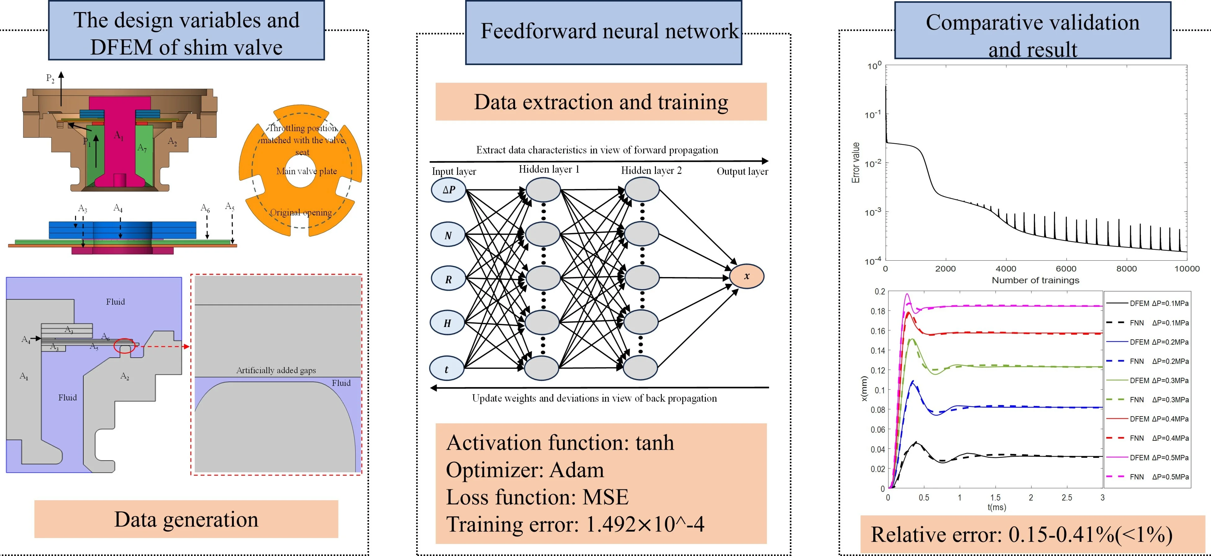
Owing to the nonlinear deformation of thin annular plates, fluid-solid coupling behaviors and complex structural combinations, dynamic characteristics of shim valves could not be captured easily in a design stage in view of traditional methods. For obtaining dynamic behaviors accurately, a dynamic finite element model (DFEM) of a shim valve in view of fluid-solid coupling is developed firstly, thus presenting dynamic features under different pressure drops and structural parameters. Utilizing the partial data from the DFEM, the FNN model is trained, and it is further used to predict other dynamic characteristics under more conditions if high accuracy of such a FNN model is available. Finally, conditions including pressure drops and diverse structural parameters for predicted results could be introduced into a DFEM, and comparisons for dynamic results from two models will be achieved, further validating feasibility of such a FNN model. It is reflected through comparisons that dynamic behaviors from the FNN model are highly consistent with those of the DFEM whether the original or predicted data is considered, and relative error for the steady-state opening is less than 1 %. Therefore, such a combination achieves a good prediction for dynamic behaviors, and it could be used to design similar valves.
Highlights
- A dynamic finite element model (DFEM) incorporating fluid-solid coupling was developed to capture the dynamic behaviors of a shim valve under diverse pressures and structural parameters.
- A feedforward neural network (FNN) was trained using DFEM data to efficiently predict the valve's complex dynamic and steady-state characteristics across multiple operating conditions.
- The hybrid DFEM-FNN approach significantly reduces computational overhead while maintaining precision, achieving a steady-state relative error of less than 1% compared to DFEM results.
- The study reveals the valve transitions from "hard" damping at low pressure differentials to "soft" damping at high differentials, providing critical insights for advanced damper design.
1. Introduction
The thin-plate structure, materials, complex boundaries, the diverse force and multi-physical field coupling problems are concentrated on a shim valve with different sizes of thin annular plates, usually characterizing geometric nonlinearity, material nonlinearity and contact nonlinearity together. It is not easy to capture behaviors of a shim valve with the complex structure in view of mathematical models. However, models and calculations for thin plates have been achieved by scholars. For example, on the basis of vibration theory of thin plates, the free vibration of thin plate with large deflection was studied by Chu [1], and the nonlinear vibration problem was solved. It was found that the modal response of the thin plate with a certain proportion of the adjacent edge length was different from that of the harmonic vibration [2]. According to the Galerkin method and the modal truncation method, the partial differential equation was simplified to the ordinary differential equation by Cockburn [3], and the concept of the integral method was also proposed. Combining the linear theory of thin plates, the incremental load technology and its formula for the bending of circular thin plates with large deflection had been developed by Q. S. Li [4], further improving the applicability and accuracy of vibration equation of thin plates by adjusting the step size in the incremental formula. Utilizing the superposition method, the nonlinear vibration for thin plates was solved by Timoshenko [5]. Considering differential quadrature method, the nonlinear free vibration of ring structure was demonstrated by J. J. Li [6]. Based on the principle of minimum potential energy, characteristics of the shim valve in a damper were presented through steady-state mathematical models by Farjoud [7], and the numerical solution with high accuracy was also obtained. Adopting the differential quadrature method, unconstrained nonlinear optimization and equivalent load method, Yuan Xianju [8, 9] and others had dealt with the partial differential equation of the thin annular plate successfully. The opening characteristics of the relief valve with thin annular plates were also obtained by them [8, 9]. Including above instances, the deflection equation of thin annular plates under static loads was usually developed and computed. The partial work was focused on steady-state behaviors of shim valves, and dynamic characteristics for the single plate and simple shim valves were also achieved. The dynamic characteristics for complex shim valves are also not easy to capture through mathematical methods at current stage.
Besides above defects in mathematical methods for shim valves, the working environment including the fluid velocity, complex pressure boundaries and the law of force transfer between plates are difficult to express accurately in a real time. Moreover, it is essentially a fluid-solid coupling problem. The finite element method is more suitable for dealing with these complex issues. For example, a two-dimensional fluid model of the centrifugal pump was established by Lang-ling [10], and the relationship between the geometric shape and the noise was also presented. The flow characteristics of a servo valve were obtained by Peng and others [11], further improving the valve structure and proposing the optimization scheme. Adopting the one-way coupling and two-way coupling manners, the excitation and vibration displacement of the centrifugal pump rotor were captured by Benra [12]. Dynamic characteristics of the fluid in bent tube and cylindrical vessel were captured by Askari and Daneshmand [13] based on the fluid-structure coupling and modal theory. A fluid-structure coupling model and the boundary element method had been proposed by Gomes [14], and the combination was successfully used to deal with the stability analysis for incompressible flow. As above instances, the fluid-structure interaction in multi-physical fields has been utilized in diverse fields. However, more instances were concentrated on the multi-step compound coupling, thus presenting defects in the characterization of fluid-solid interaction, such as complicated steps and large calculation error. For avoiding evident problems, a fully coupled method was also considered. Actually, more requirements in calculation for such a method were also evident, such as long calculation times. In a word, it is not easy to capture dynamic behaviors for all conditions in the complex structure. Fortunately, neural networks have been used to solve complex engineering problems. Of those, the feed-forward back-propagation neural network model was adopted to predict the shear capacity of anchor bolts near the edge of concrete [15]. The nonlinear transient response of the magnetopause to solar wind conditions using a neural network was obtained by Tulunay [16]. The feedforward neural network was utilized to predict water quality parameters in rivers by MJ [17].
Recent reviews [18] highlighted that machine learning (ML) provided a novel research framework. This approach demonstrated high accuracy in predicting nonlinear aerodynamic behaviors and structural responses. For instance, to accelerate fluid-solid coupling simulations via time-step prediction, a hybrid CNN-RNN surrogate model was developed by Schumacher [19]. Convolutional Auto-Encoders with LSTM networks was developed to model complex nonlinear flow fields by Hu et al. [20]. A multi-level DL-ROM framework was proposed to capture coupled nonlinear dynamics by Gupta [21]. Similarly, in gas-solid flow systems, LSTM-based models had exhibited higher accuracy in capturing flow fields compared to traditional interpolation methods [22]. Moreover, a ML-based strategy was adopted to bypass the high computational overhead of fluid-solid coupling analysis by Soni et al. [23]. A fluid-solid coupling -ML hybrid framework was developed to predict complex airflow distributions within crop canopies by Cui et al. [24]. These advancements provide a robust methodological foundation for the dynamic analysis of shim valves in this study. Specifically, the dynamic characteristics of a relief valve were obtained by a combination of fluid-solid coupling and the feedforward neural network, which provides a valuable reference for dynamic analysis of a shim valve in this paper.
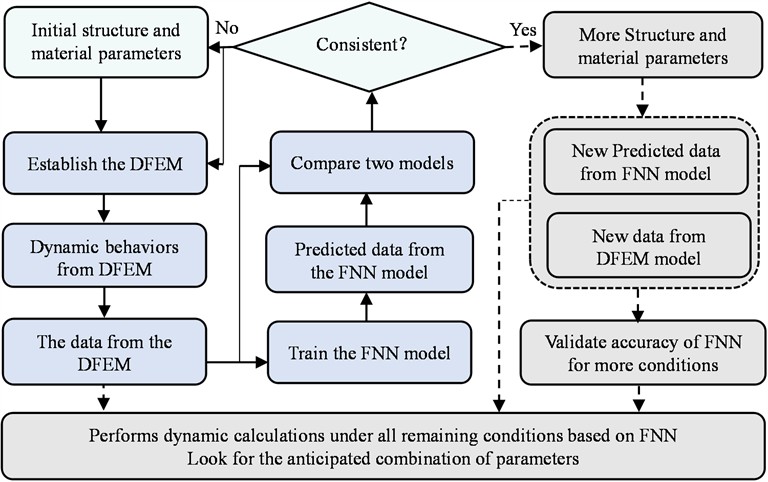
Therefore, building upon these data-driven strategies, high predictive precision will be achieved by the proposed FNN model. Compared with the original data of the DFEM, such a model will maintain a steady-state relative error of less than 1 % and reduce computational overhead. Combining the fluid-solid coupling and the feedforward neural network, the dynamic characteristics of a shim valve with several thin annular plates will be obtained gradually, and the work program is presented in Fig. 1.
Fig. 1The program for a combination of the fluid-solid coupling and the feedforward neural network
2. The details of dynamic finite element model
A typical shim vale with thin annular plates is shown in Fig. 2 [9]. Specially, it is mainly composed of seven components, such as the rivet (A1), valve seat (A2), thick valve plate group for fastening (A3), small valve plate (A4), main valve plate (A5), additional valve plate group (A6) and rib (A7) [9]. Evenly distributed along the circumference of the main valve plate, initial openings are worked as main flowing channels if the evident deflection of the main valve plate is not available. There will be an additional flow channel at the throttling position corresponding to the valve seat if the deflection of the main valve plate is caused by the pressure drop (). Such a new flow channel is associated with the pressure drop and flow rate for a given structure. The throttling area of this valve can be varied according to the pressure drop and flow rate, and the variable behavior is essentially controlled by mechanical structures.
In a word, besides material factors, the excellent performance of such a shim valve is determined by the fluid, solid and their interactions. Therefore, dynamic characteristics in view of fluid-solid coupling are considered in this paper so that the effect of crucial parameters on performance can be obtained, which is helpful for designing similar valves.
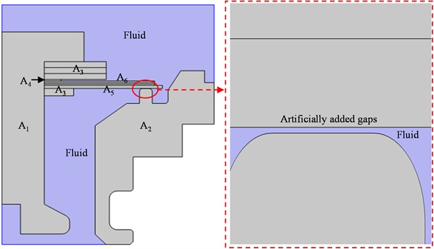
In order to reduce the number of mesh and shorten the calculation time, certain structural details will be simplified reasonably because of little effect on dynamic behaviors of main valve plate and the entire valve. For example, since the rib primarily supports the bottom of the valve and does not affect the deflection of the main valve plate, the rib can be neglected in a simulation model. The original openings of the main valve plate is not easy expressed in the simulation model. For solving such a problem, an initial throttling gap between the main valve plate and the valve seat is added to this structure, and the original openings can be canceled. This substitution is also reasonable if throttling capacity of the original openings is fully consistent with that of the artificially added gap. After simplification, such a shim valve can be expressed as a two-dimensional axisymmetric model, as shown in Fig. 3. In detail, the fluid is characterized in the blue region, and the gray area represents solid components including A1, A2, A3, A4, A5 and A6. Of these, A1, A2, A3 and A4 can be worked as fixed domains which are not moved in any direction, and the fixed restraint can be adopted directly for each component. The fixed restraint is applied to the side surfaces of A5 and A6 which are matched with the rivet, and others of them can be deformed freely under diverse fluid pressures.
Fig. 2Schematic diagram of shim valve with thin annular plates
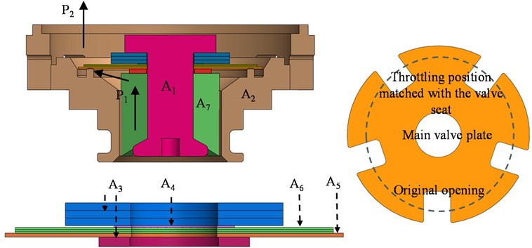
Fig. 3The two-dimensional axisymmetric model of a shim valve
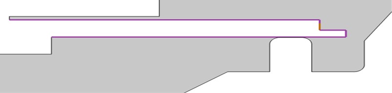
Owing to the interaction between contact surfaces of solid components, relative sliding may occur between the valve plates. In a fluid-solid coupling model, the assembly body should be adopted for such a structure, and six contact pairs between solid valve plates should be defined firstly, shown as Fig. 4. Depicted as number 7 in Fig.4, there is also a contact pair between the main valve plate and valve seat so that the penetration phenomenon can be eliminated if the main valve plate is moved downward. Besides 7 contact pairs between solid parts, there is also contact between solids and the surrounding fluid, and the uniform boundary pair is adopted between them. The relative motion of the solid boundary, the corresponding displacement field should be associated with the fluid boundary. The fluid boundary is also called a moving boundary between the solid and fluid, shown as Fig. 5. The displacement of such a boundary can be defined by the specified mesh displacement, and it is determined by the solid displacement of the uniform boundary pair.
Fig. 4The distribution of contact pairs
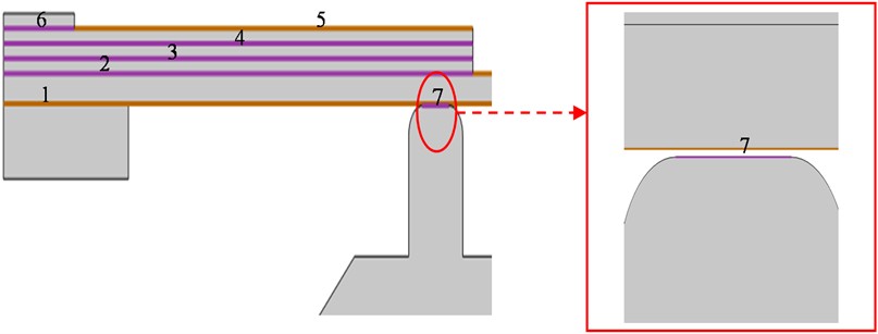
Fig. 5The moving boundary between the solid and fluid
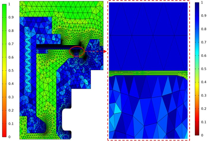
In such a two-dimensional axisymmetric model, the mesh in narrow regions should be refined. The solid areas which do not participate in deformation can be roughened, such as the rivet, valve seat, thick valve plate group for fastening and rib. Similarly, the region of fluid not near deformed plates will be also roughened. The distribution of initial finite element mesh is demonstrated in Fig. 6, which is consistent with the principle of the refinement and coarsening requirements. Specifically, the total number of mesh is 31167. The minimum element quality is close to 0.5529, and the average element quality is about 0.9235. The element area ratio is 6.775×10⁻⁶. Therefore, the mesh quality in crucial regions is high and the total number is small, which meets requirement of computation with high efficiency.
Specifically, the minimum and maximum element sizes are set to 0.0001 mm and 0.8 mm for the fluid domain, respectively. The maximum element growth rate is constrained to 1.2, with a curvature factor of 0.25. Due to the irregular geometry and thin-film characteristics of the fluid domain, a resolution of 3 is applied in narrow regions. For other domains, the minimum element size is set to 0.0003 mm with a narrow region resolution of 2, while other parameters remain consistent with those of the fluid domain.
In the assembly, the mesh nodes on both sides of the contact pair and the consistent boundary pair are discontinuous. The mesh will be stretched along the displacement direction if plates are deformed. The deformed finite element must exist in such a model as long as a relatively large displacement is generated. For these points, the mesh needs to be re-meshed at each new position.
In such a model, the fluid domain is treated as a deformable region, where the mesh can freely deform and be reconstructed. The Yeoh smoothing method is employed to handle the mesh deformation, with a specified stiffening factor of 10. Initially, the mesh deformation values in both the radial and vertical directions are set to 0. The boundaries of shims A1 through A5 are designated as the boundary conditions for the prescribed mesh displacement. All non-fluid domains and other fluid-contacting boundaries are kept strictly stationary, retaining their initial configurations. To maintain mesh quality, a dynamic remeshing trigger is established to automatically reconstruct the mesh whenever the element distortion exceeds a critical threshold of 0.5.
Fig. 6The distribution of the initial meshes
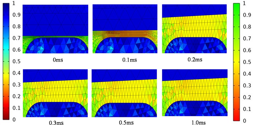
In an instance of pressure drop of 0.5 MPa, the mesh distribution of a crucial region at any time or displacement is portrayed in Fig. 7. For example, at 0.3 ms, the displacement of the main valve plate in the throttling position is 0.19 mm. The total number of mesh is 34854. The minimum element quality is 0.4998, and the average element quality is 0.8576. The element area ratio is about 8.45×10⁻⁴. For any pressure drop, the continuous computation is possible only if the mesh quality is high at any position or time.
Fig. 7The distribution of the re-meshed element in the crucial region
Completing above definitions for moving mesh model, the computation will be carried out on the basis of material parameters and solver settings. Specifically, materials are listed in Table 1. In COMSOL Multiphysics, the time unit is set to milliseconds, and the calculation time is ranged from 0 to 10 ms. The time step size is 0.01 ms if the time is varied from 0 to 1 ms, and it is 0.1 ms in other time ranges. To maintain mesh integrity under large deformation conditions, an automatic remeshing extension is integrated into the solver to update the mesh quality in real time. The transient simulation is performed by coupling four physical interfaces comprising Laminar Flow, Solid Mechanics, Moving Mesh, and fluid-solid coupling. Specifically, a fully coupled fixed geometry approach is adopted within the fluid-solid coupling module.
Table 1Material parameters [9]
Materials | Items | Parameters |
Solid | Elastic modulus | 210GPa |
Poisson’s ratio | 0.3 | |
Density | 6000 kg/m3 | |
Fluid | Dynamic viscosity | 0.01295 Pa.s |
Density | 800 kg/m3 |
Regarding the solver configuration, a segregated iterative method is employed for synchronous solution, and convergence based on a prescribed tolerance is used as the termination criterion. The maximum number of iterations is set to 100, and a tolerance factor of 0.5 is applied to achieve optimal convergence speed. All numerical tasks are performed using the MUMPS direct solver. By configuring a memory allocation factor of 1.2, the stability of large-scale matrix operations is rigorously ensured.
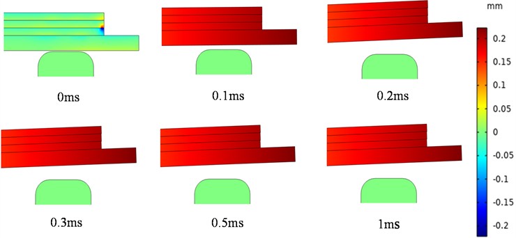
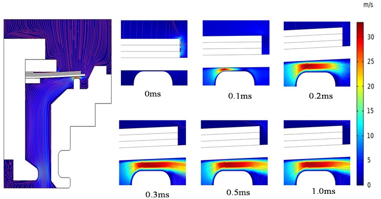
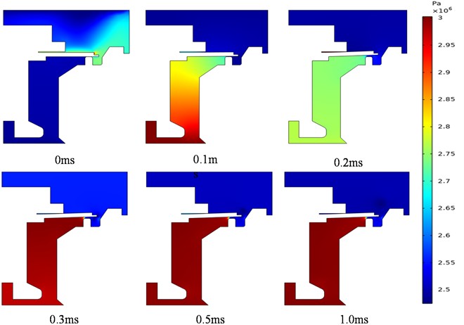
Essentially, the dynamic displacement, stress, flow rate, pressure are reflected through such a fluid-solid coupling model based on the continuous computation. For example, at a given pressure drop of 0.5 MPa, the partial dynamic variables of this structure are depicted in Figs. 8-11. It is drawn from these figures that the deflection of valve plates is changed significantly if the time is ranged from 0 to 0.3 ms. The opening size, flow speed and pressure in the throttling position are enlarged. Following the change of deflection or displacement, the stress of the valve plate is also varied. At this pressure drop, the steady-state opening of throttling position is 0.185 mm, and the maximum stress of solid components is about 644 MPa. The maximum flow velocity is 32.96 m/s.
Fig. 8The dynamic deflection of valve plates: ∆P= 0.5 MPa
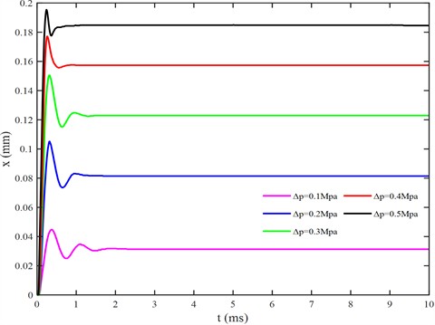
To further elucidate the dynamic response of the shim valve, the evolution of the shim deflection at the throttling position under various pressure drops is illustrated in Fig. 12. The corresponding dynamic performance metrics include response time, overshoot, and vibration frequency. These values are summarized in Table 2.
At a low pressure drop of 0.1 MPa, a characteristic underdamped oscillation is exhibited by the shim. The deflection reaches its peak at 0.43 ms and stabilizes at a steady-state value of approximately 0.03 mm after two vibration cycles (around 2 ms). As the pressure drop is increased to 0.2 MPa, the peak time is reduced to 0.33 ms. Concurrently, the overshoot and vibration frequency are significantly elevated, indicating a more rapid but volatile dynamic response. Under a moderate pressure drop of 0.3 MPa, the peak time is consistent with the 0.2 MPa case. The overshoot is further intensified and the overall response time is shortened. When subjected to high pressure drop conditions (0.4 MPa and 0.5 MPa), the vibration periodicity is significantly attenuated. Specifically, at a pressure drop of 0.5 MPa, the maximum steady-state opening is achieved within a minimum response time of approximately 0.59 ms, and the highest recorded overshoot of 0.0311 mm. No distinct oscillation cycles are observed in these cases, suggesting a transition toward an overdamped or critically damped state.
Fig. 9The varied stress of solid components following the deflection: ∆P= 0.5 MPa
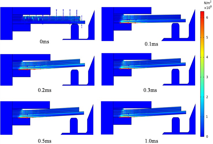
Fig. 10The flow velocity of crucial throttling region: ∆P= 0.5 MPa
In summary, an increase in the pressure drop across the shim valve leads to an expansion of the steady-state throttling opening while the response time concurrently decreases. At low pressure drops, the vibration periodicity is highly pronounced. At higher fluid loads, this periodicity is effectively attenuated. Functionally, the annular shim valve provides “hard” damping characteristics at low pressure differentials and transitions to “soft” damping at high differentials. Notably, the response time during the transition from “hard” to “soft” damping is significantly shorter, ensuring rapid adaptation to high-load conditions.
Fig. 11The pressure distribution at different times: ∆P= 0.5 MPa
To systematically investigate the influence of structural configurations on the steady-state opening and dynamic response of the annular shim valve, a parametric study is conducted within the ranges defined in Table 3.
Fig. 12Shim deflection at the throttling position under various pressure drops (P1 = 3.0 MPa)
The impact of the number of shims (N) on the deflection is illustrated in Fig. 13 (with 10.1 mm and 0.2 mm). At a constant pressure drop of 0.3 MPa, the steady-state opening is observed to decrease significantly as increases. However, the dynamic metrics such as response time, overshoot, and vibration period remain relatively consistent across different shim counts.
Table 2Dynamic characteristics of the shim valve under various pressure drops
Pressure drop (Mpa) | Response time (ms) | Overshoot (mm) | Peak time (ms) | Vibration period (ms) | Vibration frequency (HZ) |
0.1 | 1.57 | 0.0141 | 0.43 | 0.77 | 1299 |
0.2 | 1.07 | 0.0242 | 0.33 | 0.63 | 1587 |
0.3 | 0.97 | 0.0282 | 0.33 | 0.64 | 1563 |
0.4 | 0.61 | 0.0307 | 0.28 | – | – |
0.5 | 0.59 | 0.0311 | 0.26 | – | – |
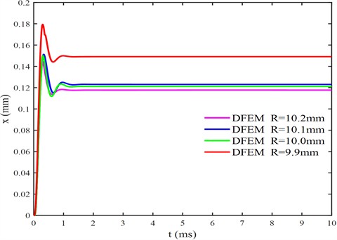
Furthermore, Fig. 14 presents the influence of the outer diameter () while keeping 4 and 0.2 mm. The maximum steady-state deflection is observed at 9.9 mm. Notably, as ranges from 10.0 mm to 10.2 mm, the deflection curves, settling time, and overshoot overlap significantly. This indicates a diminished sensitivity to diameter variations within this range.
Fig. 13Influence of the number of shims (N) on the shim deflection (pressure drop ∆P= 0.3 MPa)
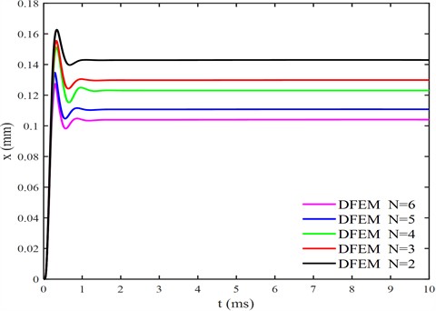
Fig. 14Influence of the shim outer diameter (R) on the shim deflection (pressure drop ∆P= 0.3 MPa)
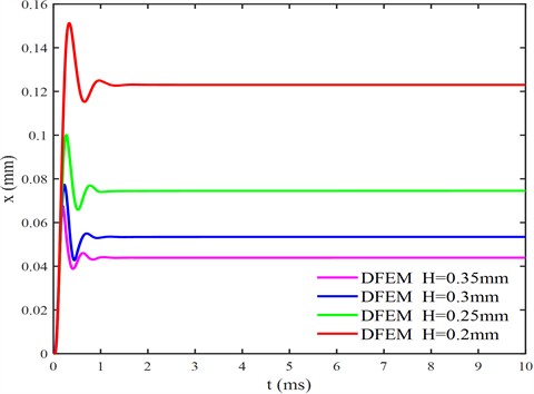
Furthermore, the effect of shim thickness () is evaluated (with 4 and 10.1 mm), as shown in Fig. 15. A clear negative correlation is identified between the steady-state opening and the shim thickness at 0.3 MPa. Despite the variations in opening size, the dynamic characteristics remain largely unaffected by , with a consistent response time of approximately 1 ms and an overshoot of 0.03 mm. In conclusion, while structural parameters and predominantly govern the steady-state throttling capacity, they exert a limited influence on the fundamental dynamic response patterns of the valve.
Table 3Parameter ranges for the structural sensitivity analysis of the shim valve
(MPa) | (mm) | (mm) | |
0.3 | 2 | 9.8 | 0.2 |
3 | 9.9 | 0.25 | |
4 | 10.0 | 0.3 | |
5 | 10.1 | 0.35 | |
6 | 10.2 | – |
Fig. 15Influence of shim thickness (H) on the shim deflection (pressure drop ∆P= 0.3 MPa)
2.1. Prediction of dynamic characteristics based on feedforward neural network (FNN)
Although the dynamic characteristics of the shim valve are accurately captured by the proposed fluid-solid coupling model, the structural optimization for specific performance targets remains a significant challenge. This limitation is primarily driven by the vast design space of diverse structural combinations and the high computational cost associated with each simulation. Specifically, the parametric combination of , , and in the study results in a total of 100 distinct operating scenarios (5×5×4). Consequently, performing high-fidelity fluid-solid coupling simulations for all these cases entails an exorbitant computational cost, which is often impractical in engineering design cycles.
Therefore, there is a compelling need for hybrid methodologies that integrate high-fidelity fluid-solid coupling models with more efficient predictive tools. Recently, the feedforward neural network has presented a good ability for predicting dynamic behaviors on the basis of fluid-solid coupling model in a similar field [25], [26]. In detail, the FNN is a computational model combined many interconnected neural units, and each neuron is able to receive input signals from others [27]. It can deal with the information in one direction, and the information can be transmitted through the input layer, hidden layer, processing layer and output layer successively [28]. Therefore, this network structure is able to express the strong nonlinearity and characterize obvious advantages for solving nonlinear problems in the field of engineering [28].
Generally, the overall accuracy of the FNN is poor if the input data are not standardized [29]. The max-min normalization manner is usually adopted in a standardization method, yielding that [30]:
in which , indicates the value of a single data, represents the original data, and denote the maximum and minimum data. A nonlinear activation function is utilized in each neuron, which is helpful to convert the input signal to the output signal. The hyperbolic tangent function (tanh) worked as the activation function can be given by [30]:
where signifies the input signal. The output result of this function is ranged from –1 to 1, and it is able to deal with negative information.
In addition to utilization of the activation function, the number of neurons in the input layer, the hidden layer and the output layers should be considered in this model. The FNN in this instance has four layers, shown as an input layer, an output layer and two hidden layers in Fig. 16.
Fig. 16Schematic of the FNN structure
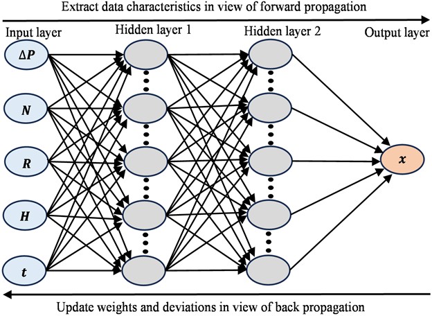
Specifically, the pressure drop (), number of valve plates (), radius of main valve plate (), thickness of main valve plate () and time () are characterized in the input layer. The deflection or displacement () of the main valve plate at the throttling position is associated with the output layer. The number of neurons in both hidden layers is limited to 100. The data set utilized to train the FNN is shown in Table 4. The time is varied from 0 to 10 ms.
In the FNN model, there is a difference between the predicted result and the original data from the DFEM, and it can be further measured by a loss function. The predicted value will be consistent with the original ones if the result of the loss function is small enough [31]. The training process can be ended as long as the smaller value of the loss function has been achieved [32]. Generally, the loss function for the regression problem can be followed that [33]:
where is the number of samples, represents the original result, denotes the predicted value.
During error backpropagation, the torch.nn.MSELoss.backward method is utilized to compute the gradients [34]. Based on the torch.optim.Adam algorithm [34], an Adam optimizer is configured to iteratively update the model parameters. The specific hyperparameters of the proposed FNN model are summarized in Table 5.
Following the architecture setup and data normalization, the FNN is trained through a systematic iterative process. During each training epoch, the network gradients are initially zeroed to prevent unintended accumulation. Forward propagation is executed by feeding the normalized input data into the model to generate predictions. Subsequently, the deviation between the predictions and the DFEM benchmarks is computed via the MSE loss function, followed by backpropagation to calculate gradients. Finally, the model weights are updated using the Adam optimizer based on the obtained gradients.
Table 4The data set utilized to train the FNN
(MPa) | (mm) | (mm) | (MPa) | (mm) | (mm) | ||
0.1 | 2 | 9.9 | 0.2 | 0.3 | 4 | 10.0 | 0.3 |
0.25 | 10.1 | 0.2 | |||||
0.3 | 0.25 | ||||||
10.0 | 0.2 | 0.3 | |||||
0.25 | 6 | 9.9 | 0.2 | ||||
0.3 | 0.25 | ||||||
10.1 | 0.2 | 0.3 | |||||
0.25 | 10.0 | 0.2 | |||||
0.3 | 0.25 | ||||||
4 | 9.9 | 0.2 | 0.3 | ||||
0.25 | 10.1 | 0.2 | |||||
0.3 | 0.25 | ||||||
10.0 | 0.2 | 0.3 | |||||
0.25 | 0.5 | 2 | 9.9 | 0.2 | |||
0.3 | 0.25 | ||||||
10.1 | 0.2 | 0.3 | |||||
0.25 | 10.0 | 0.2 | |||||
0.3 | 0.25 | ||||||
6 | 9.9 | 0.2 | 0.3 | ||||
0.25 | 10.1 | 0.2 | |||||
0.3 | 0.25 | ||||||
10.0 | 0.2 | 0.3 | |||||
0.25 | 4 | 9.9 | 0.2 | ||||
0.3 | 0.25 | ||||||
10.1 | 0.2 | 0.3 | |||||
0.25 | 10.0 | 0.2 | |||||
0.3 | 0.25 | ||||||
0.3 | 2 | 9.9 | 0.2 | 0.3 | |||
0.25 | 10.1 | 0.2 | |||||
0.3 | 0.25 | ||||||
10.0 | 0.2 | 0.3 | |||||
0.25 | 6 | 9.9 | 0.2 | ||||
0.3 | 0.25 | ||||||
10.1 | 0.2 | 0.3 | |||||
0.25 | 10.0 | 0.2 | |||||
0.3 | 0.25 | ||||||
4 | 9.9 | 0.2 | 0.3 | ||||
0.25 | 10.1 | 0.2 | |||||
0.3 | 0.25 | ||||||
10.0 | 0.2 | 0.3 | |||||
0.25 |
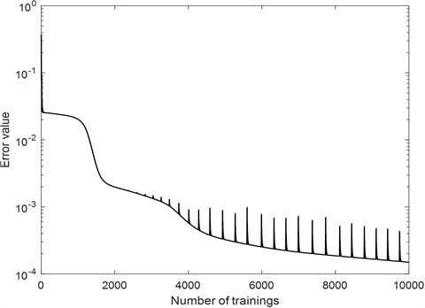
A repetitive process of forward and backward propagation in the FNN model will be ended once the error is close to the defined minimum value. In this instance, the error value of neural network extraction is approached to the minimum after 10000 epochs. During the training process, the distribution of error is shown in Fig. 17. In order to evaluate the error value of neural network calculation during training, the -axis scale in Fig. 17 can be logarithmic. At the 10000th epoch, the corresponding error is close to 1.492×10⁻⁴, and it meets the requirement for error, thus completing the training process.
The data has been normalized for training the FNN model conveniently. The output data drawn from the FNN model should be de-normalization so that anticipated results of deflection and others can be extracted directly. The de-normalization expression is followed that [30]:
in which is de-normalization result, represents predicted value, and denote the maximum and minimum values of the data in the training sample.
Table 5Hyperparameters of the FNN model
Hyperparameter | Value |
Number of layers | 4 |
Neurons per layer | [5 100 100 1] |
Learning rate | 0.001 |
batch size | 10000 |
Loss function | MSE (mean square error) |
Activation function | Tanh |
Optimizer | Adam (adaptive moment estimation) |
Fig. 17The distribution of error during the training process
Completing the above processes, comparisons for results of DFEM and FNN will be carried out, and the predicted ability can be evaluated by values of two models. For diverse pressure drops and the same structure, predicted results of the FNN model and the original data from the DFEM are portrayed in Fig. 18. It is evidently concluded from comparisons that the response time from two models is less than 2 ms. The peak time and vibration frequency are also consistent with each other. In results of the FNN model, the steady-state deflection or displacement are 0.03215 mm, 0.08211 mm, 0.1235 mm, 0.1575 mm and 0.1848 mm respectively. Compared with original data from the DFEM, relative errors are 0.15 %, 0.21 %, 0.41 %, 0.19 %, 0.27 %. Therefore, the accuracy of such a FNN model is high enough for estimating dynamic behaviors under more conditions. The predicted instances in view of diverse structural parameters are demonstrated in Figs. 19-21.
Fig. 18Comparisons for deflection drawn from two models under different pressure drops: N= 4, R= 10.1 mm, H= 0.2 mm
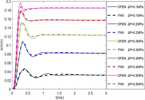
Fig. 19Comparisons for deflection drawn from two models under different numbers of valve plate: ΔP= 0.3 MPa, R= 10.1 mm, H= 0.2 mm
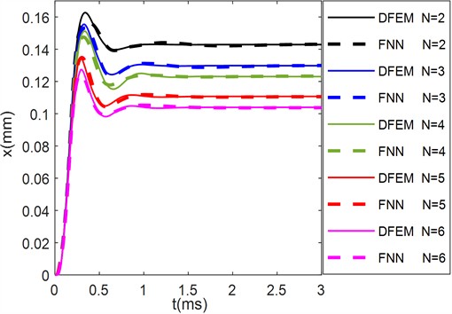
Fig. 20Comparisons for deflection drawn from two models under different radius of main valve plate: ΔP= 0.3 MPa, N= 4, H= 0.2 mm
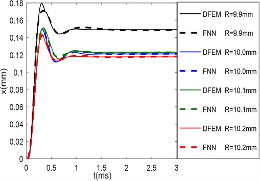
Evidently, the dynamic curves of the FNN model are consistent with those of the DFEM. The errors for the response time, overshoot and steady-state value are very small. Therefore, the FNN model can also be used to capture dynamic characteristics under different structural parameters.
Fig. 21Comparisons for deflection drawn from two models under different thickness of main valve plate: ΔP= 0.3 MPa, N= 4, R= 10.1 mm
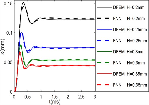
In summary, superior nonlinear modeling capabilities are demonstrated by the FNN model. The steady-state opening and dynamic response characteristics of annular shim valves are accurately characterized across a wide range of parameters, including varying pressure drops, number of shims, and geometric dimensions (outer radius and thickness). The reliability of the model is validated by the minimal discrepancies observed between the FNN predictions and the high-fidelity DFEM simulation benchmarks. By replacing computationally intensive fluid-solid coupling simulations with this efficient surrogate model, the efficiency of valve system parameter design and structural optimization is dramatically accelerated.
3. Conclusions
On the basis of a dynamic finite element model (DFEM), dynamic characteristics of a shim valve under diverse pressure drops and structural parameters have been obtained, which are followed that:
1) With the increase of the pressure drop, the steady-state opening of the valve is enlarged. The overshoot is also increased. The response time, peak time and period of vibration are reduced under this condition. The effect of pressure drop on dynamic behavior is relatively evident. Specifically, at a pressure drop of 0.5 MPa, the valve achieves a steady-state opening of 0.185 mm and a maximum flow velocity of 32.96 m/s, with the peak stress of 644 MPa remaining within the structural safety margin.
2) A clear transition in the damping performance of the valve is revealed by the results. Low pressure differentials yield “hard” damping characteristics with high stiffness and low flow. Rising differentials induce a shift toward “soft” damping with increased flexibility and higher flow. Such a transition is critical for advanced damper design. It ensures superior low-speed stability and high-speed impact absorption, effectively balancing ride comfort and vehicle handling.
3) The influence of structural parameters on dynamic characteristics is relatively insensitive, such as the radius, number and thickness. However, steady-state indexes such as the opening is highly associated with structural parameters. For example, there is a negative correlation between the steady-state opening and the structural parameters including the number and thickness, the influence of the radius of the main valve plate on the steady-state opening is nonlinear.
4) While dynamic characteristics has been captured by the DFEM, the disadvantages of long calculation time, high modeling complexity and poor generality also exist. Therefore, the FNN model is established based on the partial data from the DFEM, and dynamic results of such a simple artificial intelligence model are highly consistent with those of DFEM. Compared with original data of the DFEM, the relative error of steady-state results generated by the FNN model is less than 1 %. Therefore, the proposed FNN model presents a good ability for estimating dynamic and steady-state behaviors under diverse combination of conditions, such as pressure drop, number of valve plate, radius of main valve plate and thickness of main valve plate.
Such a combining method with the DFEM and FNN model can be used to deal with shim valves with thin annular plates, thus fusing advantages of high precision, short calculation time and low requirement of calculation conditions. The parameter design efficiency and optimization of this type of system can be improved based on such a combination.
References
-
H.-N. Chu and G. Herrmann, “Influence of large amplitudes on free flexural vibrations of rectangular elastic plates,” Journal of Applied Mechanics, Vol. 23, No. 4, pp. 532–540, Dec. 1956, https://doi.org/10.1115/1.4011396
-
K. Yasuda, T. Torii, and M. Kasahara, “Proposition of an incremental transfer matrix method for nonlinear vibration analysis,” JSME International Journal, Series III: Vibration, Control Engineering, Engineering for Industry, Vol. 34, No. 1, pp. 12–18, Mar. 1991, https://doi.org/10.1299/jsmec1988.34.12
-
B. Cockburn, “Discontinuous Galerkin methods,” ZAMM – Journal of Applied Mathematics and Mechanics / Zeitschrift für Angewandte Mathematik und Mechanik, Vol. 83, No. 11, pp. 731–754, Nov. 2003, https://doi.org/10.1002/zamm.200310088
-
Q. S. Li, J. Liu, and H. B. Xiao, “A new approach for bending analysis of thin circular plates with large deflection,” International Journal of Mechanical Sciences, Vol. 46, No. 2, pp. 173–180, Feb. 2004, https://doi.org/10.1016/j.ijmecsci.2004.03.012
-
S. P. Timoshenko and J. M. Gere, Theory of Elastic Stability. Courier Corporation, 2012.
-
J.-J. Li and C.-J. Cheng, “Differential quadrature method for nonlinear vibration of orthotropic plates with finite deformation and transverse shear effect,” Journal of Sound and Vibration, Vol. 281, No. 1-2, pp. 295–309, Mar. 2005, https://doi.org/10.1016/j.jsv.2004.01.016
-
A. Farjoud, M. Ahmadian, M. Craft, and W. Burke, “Nonlinear modeling and experimental characterization of hydraulic dampers: effects of shim stack and orifice parameters on damper performance,” Nonlinear Dynamics, Vol. 67, No. 2, pp. 1437–1456, Jun. 2011, https://doi.org/10.1007/s11071-011-0079-2
-
X. Yuan, T. Tian, H. Zhou, and J. Zhou, “Comparisons of methods for solving static deflections of a thin annular plate,” Applied Numerical Mathematics, Vol. 127, pp. 266–279, May 2018, https://doi.org/10.1016/j.apnum.2018.01.012
-
X. Yuan and K. Guo, “Modelling and analysis for a pilot relief valve using CFD method and deformation theory of thin plates,” Science China Technological Sciences, Vol. 58, No. 6, pp. 979–998, Apr. 2015, https://doi.org/10.1007/s11431-015-5822-3
-
L. L. Zeng, X. D. Lai, X. M. Chen, D. X. Ye, D. M. Song, and G. L. Liao, “The effect of the blade tip clearance on the internal flow characteristics of the double-blade semi-open impeller submersible sewage pump,” China Rural Water and Hydropower, No. 5, pp. 51–57, May 2022.
-
J. Peng, Y. Zhang, S. Li, W. Bao, and Y. Tanaka, “Identification algorithm and improvement of modal damping ratios for armature assembly in a hydraulic servo-valve with magnetic fluid,” Energies, Vol. 16, No. 8, p. 3419, Apr. 2023, https://doi.org/10.3390/en16083419
-
F.-K. Benra, H. J. Dohmen, J. Pei, S. Schuster, and B. Wan, “A comparison of one-way and two-way coupling methods for numerical analysis of fluid-structure interactions,” Journal of Applied Mathematics, Vol. 2011, No. 1, p. 853560, Mar. 2011, https://doi.org/10.1155/2011/853560
-
E. Askari and F. Daneshmand, “Coupled vibration of a partially fluid-filled cylindrical container with a cylindrical internal body,” Journal of Fluids and Structures, Vol. 25, No. 2, pp. 389–405, Feb. 2009, https://doi.org/10.1016/j.jfluidstructs.2008.07.003
-
J. P. Gomes and H. Lienhart, “Fluid-structure interaction-induced oscillation of flexible structures in laminar and turbulent flows,” Journal of Fluid Mechanics, Vol. 715, pp. 537–572, Jan. 2013, https://doi.org/10.1017/jfm.2012.533
-
M. A. Alqedra and A. F. Ashour, “Prediction of shear capacity of single anchors located near a concrete edge using neural networks,” Computers and Structures, Vol. 83, No. 28-30, pp. 2495–2502, Nov. 2005, https://doi.org/10.1016/j.compstruc.2005.03.019
-
Y. Tulunay, D. G. Sibeck, E. T. Senalp, and E. Tulunay, “Forecasting magnetopause crossing locations by using neural networks,” Advances in Space Research, Vol. 36, No. 12, pp. 2378–2383, Jan. 2005, https://doi.org/10.1016/j.asr.2004.04.015
-
M. J. Diamantopoulou, D. M. Papamichail, and V. Z. Antonopoulos, “The use of a neural network technique for the prediction of water quality parameters,” Operational Research, Vol. 5, No. 1, pp. 115–125, Jan. 2005, https://doi.org/10.1007/bf02944165
-
Z. Zhang et al., “Advances in machine learning for wind-induced fluid-structure interaction of large-scale structures,” (in Chinese), Acta Aerodynamica Sinica, Vol. 43, No. 5, pp. 53–77, May 2025, https://doi.org/10.7638/kqdlxxb-2025.0061
-
A. Schumacher, “Machine learning of fluid-structure interaction,” University of Stuttgart, 2021, https://doi.org/10.18419/opus-11886
-
J. Hu, Z. Dou, and W. Zhang, “Fast fluid-structure interaction simulation method based on deep learning flow field modeling,” Physics of Fluids, Vol. 36, No. 4, p. 047118, Apr. 2024, https://doi.org/10.1063/5.0200188
-
R. Gupta, “Deep learning-based reduced order modeling for unsteady flow dynamics and fluid-structure interaction,” University of British Columbia, Vol. 34, No. 3, 2022, https://doi.org/10.1063/5.0082741
-
S. Li, G. Duan, and M. Sakai, “On reduced-order modeling of gas-solid flows using deep learning,” Physics of Fluids, Vol. 36, No. 3, p. 033333, Mar. 2024, https://doi.org/10.1063/5.0193480
-
T. Soni, A. Sharma, R. Dutta, A. Dutta, S. Jayavelu, and S. Sarkar, “Capturing functional relations in fluid-structure interaction via machine learning,” Royal Society Open Science, Vol. 9, No. 4, p. 211516, Apr. 2022, https://doi.org/10.1098/rsos.220097
-
H. Cui, C. Wang, X. Liu, X. Liu, J. Yuan, and Y. Liu, “Prediction of the distribution of airflow within the cotton canopy using fluid-structure interaction simulation and machine-learning methods,” Biosystems Engineering, Vol. 232, pp. 51–66, Aug. 2023, https://doi.org/10.1016/j.biosystemseng.2023.06.011
-
C. Wang, X. Yuan, J. Chen, X. Chen, and T. Qiu, “Dynamic characteristics of a relief valve captured by a combination of fluid-solid coupling and feedforward neural network (FNN),” Transactions of the Canadian Society for Mechanical Engineering, Vol. 48, No. 2, pp. 253–266, Jun. 2024, https://doi.org/10.1139/tcsme-2023-0116
-
H. Von Wahl and T. Richter, “Using a deep neural network to predict the motion of underresolved triangular rigid bodies in an incompressible flow,” International Journal for Numerical Methods in Fluids, Vol. 93, No. 12, pp. 3364–3383, Aug. 2021, https://doi.org/10.1002/fld.5037
-
G. Bebis and M. Georgiopoulos, “Feed-forward neural networks,” IEEE Potentials, Vol. 13, No. 4, pp. 27–31, Oct. 1994, https://doi.org/10.1109/45.329294
-
D. Svozil, V. Kvasnicka, and J. Pospichal, “Introduction to multi-layer feed-forward neural networks,” Chemometrics and Intelligent Laboratory Systems, Vol. 39, No. 1, pp. 43–62, Nov. 1997, https://doi.org/10.1016/s0169-7439(97)00061-0
-
Y. Xie and M. A. Jabri, “Training algorithms for limited precision feedforward neural networks,” Technical Report, Vol. 8, No. 3, 1991.
-
T. L. Fine, Feedforward Neural Network Methodology. New York: Springer-Verlag, 1999, https://doi.org/10.1007/b97705
-
C. Alippi, “Selecting accurate, robust, and minimal feedforward neural networks,” IEEE Transactions on Circuits and Systems I: Fundamental Theory and Applications, Vol. 49, No. 12, pp. 1799–1810, Dec. 2002, https://doi.org/10.1109/tcsi.2002.805710
-
D. J. Montana and L. Davis, “Training feedforward neural networks using genetic algorithms,” in Proceedings of the 11th International Joint Conference on Artificial Intelligence (IJCAI), Vol. 89, No. 1, pp. 762–767, Aug. 1989.
-
P. Patrick van der Smagt, “Minimisation methods for training feedforward neural networks,” Neural Networks, Vol. 7, No. 1, pp. 1–11, Jan. 1994, https://doi.org/10.1016/0893-6080(94)90052-3
-
A. Paszke et al., “Automatic differentiation in PyTorch,” in Proceedings of the 31st Conference on Neural Information Processing Systems (NIPS), pp. 1–4, 2017.
About this article

The authors gratefully acknowledge that the work described here was financially supported by the National Natural Science Foundation of China (No. 51605149) and the Zhongyuan Sci-Tech Innovation Leading Talents (grant No. 244200510045). This work was also sponsored by the Excellent Youth Fund of Hubei University of Automotive Technology (No. 2023YQ04). Qixin Zhu and Lifeng Wei worked equally, and they are co-first authors.
The datasets generated during and/or analyzed during the current study are available from the corresponding author on reasonable request.
Qixin Zhu: investigation, methodology. Lifeng Wei: writing-original draft. Xianju Yuan and Zhongqiang Feng: writing-review and editing. Yaohua Guo: supervision
The authors declare that they have no conflict of interest.

