Circuit breaker sound source localization method based on cross-channel attention fusion

Gu, Guangmin; Zhang, Wei; Wan, Fei; Zhao, Like

doi:10.21595/jve.2026.26265

Journal of Vibroengineering

Browse Journal

Submit article

Published: August 3, 2026

Check for updates

Circuit breaker sound source localization method based on cross-channel attention fusion

Guangmin Gu¹

Wei Zhang²

Fei Wan³

Like Zhao⁴

^{1, 2, 3, 4}Inner Mongolia Power (Group) Co., Ltd., Ordos Power Supply Branch, Ordos 017000, Inner Mongolia, China

Corresponding Author:

Guangmin Gu

Cite the article Download PDF

Article in Press

Downloads 0

Abstract

Identifying the active circuit breaker in densely packed distribution cabinets is challenging, as acoustic signatures from neighboring breakers often overlap. At the same time, microphone-array-based localization remains expensive to deploy. To address these limitations, we propose a stereo-enhanced cross-channel attention framework that localizes the source using only a fixed dual-microphone recorder. The input is represented as a six-channel time-frequency feature map that combines left and right log-Mel spectrograms, interaural level difference (ILD), interaural phase difference (IPD) encoded as cosine and sine components, and a GCC-PHAT peak map, enabling a clear separation between content and spatial cues. On top of this representation, we introduce Stereo-Enhanced Cross-Channel Attention (SECCA), in which the content branch provides Query features while the spatial branch provides Key and Value features for cross-channel guidance. The module injects directional information into content modeling through lightweight global pooling and gating. The resulting features are fed into a ConvNeXt-T backbone with hierarchical dual-head supervision for coarse region classification and fine breaker classification, with only the fine head retained during inference. File-level predictions are obtained by averaging clip-level posteriors within each recording. On a 10-kV switchgear dataset comprising 900 recordings across nine breaker positions, two operation types, and five load-current levels, ConvNeXt-T + SECCA achieves a file-level Macro-F1 of 84.79 %±2.26 % (+4.10 points) and a file-level localization accuracy of 84.90 %, with a peak of 88.00 %. Attention visualization and LR-swap consistency analysis further show that SECCA learns frequency-selective and spatially informative responses, rather than acting as a simple parameter increase. These results indicate that the proposed method provides a non-contact, low-cost solution for on-site cabinet inspection and online maintenance. The reported performance should be interpreted under a controlled fixed-recorder geometry.

1. Introduction

Distribution cabinets are critical assets in field power distribution and protection systems. The operating state of a circuit breaker directly affects supply reliability and maintenance efficiency [1]. As a result, online condition monitoring has attracted sustained attention, with representative approaches based on vibration sensing [2], abnormal current analysis [3], and infrared inspection [4]. However, these methods typically require additional sensors and wiring, leading to nontrivial deployment cost and sensitivity to site conditions. In contrast, acoustic fingerprinting enables non-contact sensing with high sensitivity and low installation overhead, making it well suited to routine inspection in distribution rooms [5].

Most acoustic studies on circuit breakers have focused on mechanical fault diagnosis, that is, determining whether a breaker is healthy or faulty [6]. In practice, however, operators also need to determine which breaker generated a given operation sound or abnormal acoustic event. This in-cabinet localization task becomes particularly challenging in densely populated cabinets: acoustic signatures from adjacent breakers overlap, multiple devices may operate within a short time window, and the confined space limits sensor placement. Conventional array-based localization methods (e.g., beamforming or TDOA triangulation) often require a dedicated microphone aperture around the target area, which increases installation cost and reduces portability [10], [19].

Deep audio classifiers typically begin with log-Mel spectrograms to capture spectral content [7]. To incorporate spatial information, multi-channel audio processing often relies on phase-aware representations, including complex-valued spatial features [8]. For binaural recordings, interaural level difference (ILD) and interaural phase difference (IPD) are widely used to encode direction-dependent cues [9], and learning-based sound source localization has shown robustness under interference [10]. In addition, generalized cross-correlation (GCC) provides a lightweight estimate of inter-channel time delay and remains effective for capturing TDOA information [11]. Recent studies on power equipment monitoring further indicate that modern backbones such as ConvNeXt perform well on time-frequency representations [12].

Motivated by joint-loss training in multi-task distillation [13] and multi-representation fusion strategies [14], we develop an attention-guided fusion framework for breaker sound source localization. Prior work has combined residual networks with channel attention to improve spatial discrimination [15]. Our model adopts ConvNeXt-T [16], which incorporates key design ideas from Transformers [17], and integrates lightweight channel gating similar to squeeze-and-excitation [18]. This approach is consistent with prior work on joint localization-and-detection learning in audio [19] and is further motivated by recent advances in robust GCC-based time-delay estimation, including CNN-parameterized GCC-PHAT features [20] and sub-band GCC representations [21].

To address the challenges above, we propose a stereo-enhanced cross-channel attention framework that localizes circuit breaker operation sounds using only a fixed dual-microphone recorder. The core idea is to explicitly separate content and spatial cues and then use spatial information to guide content modeling through cross-channel attention. Our main contributions are summarized as follows:

(1) We propose a Stereo-Enhanced Cross-Channel Attention (SECCA) module in which the content branch supplies Query features, while the spatial branch supplies Key and Value features for cross-channel guidance. This design uses stereo spatial cues to guide content modeling through lightweight global pooling and gating while keeping the module computationally efficient.

(2) We design a physically interpretable six-channel stereo representation by stacking left/right log-Mel spectrograms with ILD, IPD (cos/sin), and a GCC-PHAT peak map. The representation aligns content and spatial information in a unified time-frequency domain and provides structured inputs for SECCA.

(3) We employ hierarchical dual-head supervision that jointly optimizes coarse region classification and fine breaker classification during training, while retaining only the fine head at inference. This strategy improves training stability without increasing inference cost.

2. Audio data acquisition and acoustic modeling

2.1. Experimental setup and procedure

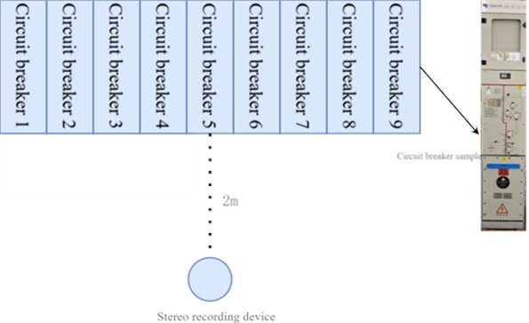
Audio data were collected from a 10-kV switchgear cabinet in a distribution-room environment. Since a typical distribution room contains 8-12 cubicles, we selected nine cubicles for the localization study and indexed them from left to right as 1-9. This configuration provides sufficient spatial variation while mitigating class ambiguity caused by overly dense spacing.

A fixed dual-microphone stereo recorder was used to acquire audio at 48 kHz. The recorder was fixed 2 m in front of breaker No. 5, which satisfies safety constraints while maintaining a practical signal-to-noise ratio. The experimental layout is shown in Fig. 1.

The recorder placement was kept fixed throughout this study to match the intended inspection scenario and to control the acoustic geometry during model comparison. Therefore, the reported results should be interpreted as performance under this fixed geometry rather than as evidence of full invariance to arbitrary microphone placements. To reduce overfitting to minor stereo perturbations, training used left-right channel swapping, ILD jitter, and ITD jitter; however, multi-placement validation remains an important direction for future work.

Fig. 1Schematic diagram of the audio recording experiment. The original photograph was taken by Guangmin Gu at the High-Voltage Laboratory, Nanjing Institute of Technology, Nanjing, Jiangsu, China, on November 20, 2025

Schematic diagram of the audio recording experiment. The original photograph was taken by Guangmin Gu at the High-Voltage Laboratory, Nanjing Institute of Technology, Nanjing, Jiangsu, China, on November 20, 2025

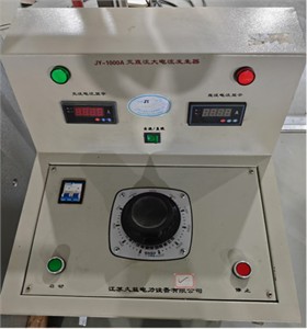
For each breaker position, two operations (opening and closing) were recorded under five load-current levels: 0 %, 20 %, 50 %, 80 %, and 100 % of rated current (0 A, 126 A, 315 A, 500 A, and 630 A). Each operation was repeated five times. The high-current generator used in the experiments is shown in Fig. 2.

Fig. 2High-current generator. The original photograph was taken by Guangmin Gu at the High-Voltage Laboratory, Nanjing Institute of Technology, Nanjing, Jiangsu, China, on November 20, 2025

High-current generator. The original photograph was taken by Guangmin Gu at the High-Voltage Laboratory, Nanjing Institute of Technology, Nanjing, Jiangsu, China, on November 20, 2025

In total, 900 recordings were collected. Each filename encodes the breaker position, load current, operation type, and trial index, separated by underscores (e.g., Position1_500A_closing_01 denotes the first closing recording of breaker 1 at 500 A).

2.2. Feature extraction method for circuit-breaker acoustic fingerprints

Breaker opening and closing events vary substantially in duration, and the raw recordings range from 2 to 12 s. To satisfy the fixed-input requirement of the model while increasing sample diversity, we segmented each recording into 2-s clips using a sliding window (window length: 2 s; hop size: 1 s; 50 % overlap), resulting in 2-9 clips per recording. We then removed silent segments with an energy-based filter by discarding clips whose RMS level was below –35 dBFS, leaving approximately 3,300 valid clips. Each clip was assigned the breaker-position label of its source recording.

2.3. Stereo acoustic fingerprint feature extraction

We adopt log-Mel spectrograms to model spectral content [7]. Since log-Mel features do not encode phase explicitly, we augment them with binaural spatial cues. Specifically, we compute ILD and IPD (cos/sin) as commonly used interaural features [9], and we compute GCC-PHAT to capture time-delay information between the two channels [11]. These complementary cues enable the network to exploit both content and direction-dependent information in a unified time-frequency representation.

For an input stereo audio clip, let $s_{L} (t)$ and $s_{R} (t)$ denote the time-domain waveforms of the left and right channels, respectively. Each clip ( $y$ ) contains ( $L =$ 96000) samples and we apply the short-time Fourier transform (STFT) separately to the two channels:

1

\begin{matrix} S_{L / R} (f, n) = \sum_{k = 0}^{N - 1} s_{L / R} (n \cdot H + k) w (k) e^{- j 2 π f k / N} \end{matrix},

where $N =$ 2048 is the window length (approximately 43 ms), $H =$ 512 is the hop size, $w (k)$ is the Hann window, $n$ is the frame index, $f \in {0, \dots, N - 1}$ is the frequency index, and $k \in {0, \dots, N - 1}$ is the sample index within a frame. For a 2 s audio clip with $L$ = 96000 samples, the number of STFT frames depends on the boundary handling strategy, as given in Eq. (2):

2

\begin{matrix} T_{o r i g i n a l} = ⌊\frac{L - N}{H}⌋ + 1 = 184 \end{matrix} .

In implementation, zero-padding is applied so that the final analysis window fully covers the signal tail, resulting in 185 STFT frames for a 2-s clip. To standardize the network input size, all feature maps are then linearly resampled along the time axis to 128 frames:

3

\begin{matrix} X (f, t^{'}) = {I n t e r p}_{t}^{(128)} X (f, t), t^{'} = 1, \dots, 128 \end{matrix},

where $I n t e r p (\cdot)$ denotes the linear interpolation operator. On this basis, the following six feature channels are extracted:

(1) Left-channel log-Mel spectrogram: the STFT magnitude spectrum $| S_{L} (f, t) |$ is projected onto the Mel scale using a bank of 128 Mel filters. The Mel filter bank is defined as a set of triangular filters $H_{m} (f)$ ( $m \in \{1, \dots, 128\}$ is the Mel band index). For each time frame, the Mel-band energy is computed as:

4

\begin{matrix} S_{L}^{m e l} (m, t) = \sum_{f = 0}^{N - 1} {| S_{L} (f, t) |}^{2} \cdot H_{m} (f) \end{matrix} .

Followed by logarithmic compression and temporal interpolation to obtain:

5

\begin{matrix} X_{L}^{m e l} (m, t^{'}) = l o g (S_{L}^{m e l} (m, t) + ϵ), ϵ = 10^{- 6} \end{matrix} .

(2) Right-channel log-Mel spectrogram: analogously, the right-channel log-Mel spectrogram is computed, yielding $X_{R}^{m e l} \in R^{128 \times 128}$ .

(3) Inter-channel level difference (ILD): ILD is defined as the logarithmic ratio of energies between the left and right channels on the Mel scale. Since $S_{L}^{m e l} (m, t)$ is already an energy measure, ILD is computed directly as the decibel value of the energy ratio:

6

\begin{matrix} X_{I L D} (m, t) = 10 {l o g}_{10} \frac{S_{L}^{m e l} (m, t) + ϵ}{S_{R}^{m e l} (m, t) + ϵ} \end{matrix} .

(4) Cosine component of the phase difference: phase-difference information is first computed at the STFT frequency-bin level and then resampled along the frequency axis to 128 frequency units. Specifically, the phase difference between the complex STFT spectra of the left and right channels is calculated as:

7

\begin{matrix} Δ ϕ (f, t) = ∠ S_{L} (f, t) - ∠ S_{R} (f, t) \end{matrix},

where $∠ S (f, t)$ denotes the phase angle of the complex STFT spectrum. The frequency dimension is then resampled to 128 equally spaced units: if the number of STFT frequency bins exceeds 128, the first 128 bins are retained; if it is fewer than 128, bilinear interpolation is used to upsample. The cosine component of the phase difference is thus obtained as:

8

\begin{matrix} X_{{I P D}_{c o s}} (i, t) = c o s (Δ ϕ_{r e s a m p} (i, t)), i \in {1, \dots, 128} \end{matrix} .

(5) Similarly, the sine component of the phase difference is obtained as:

9

\begin{matrix} X_{I P D_s i n} (i, t) = s i n (Δ ϕ_{r e s a m p} (i, t)) \end{matrix} .

The cosine and sine components of the IPD jointly encode the binaural phase-difference information, which is particularly important for azimuth discrimination of low-frequency sounds. To avoid numerical discontinuities caused by phase wrapping, the IPD is represented by its cosine and sine components rather than by the raw phase angle. Such binaural cues are widely used in learning-based sound event localization and detection frameworks [19].

(6) GCC-PHAT peak: for each time frame ( $t$ ), the generalized cross-correlation function between the left and right channels is computed as:

10

\begin{matrix} R_{L R} (τ, t) = I F F T [\frac{S_{L} (f, t) \cdot S_{R}^{*} (f, t)}{| S_{L} (f, t) \cdot S_{R}^{*} (f, t) |}] \end{matrix},

where $τ$ is the time-delay variable and $t$ is the time-frame index. Since the spacing between the two phone microphones is only about 1.5-2 cm, the maximum physical delay is approximately 0.04-0.06 ms, so only the range $τ \in [- 5,5]$ of the cross-correlation function is retained. The $τ$ -axis is then linearly resampled to 128 lag units and aligned along the time dimension to 128 frames, yielding a tensor in which the location of the GCC peak directly corresponds to the horizontal azimuth of the sound source [11]. Recent work improves GCC-based TDOA estimation under noise and reverberation via CNN-based parametrized GCC-PHAT features [20] and sub-band GCC representations [21].

The above six channels are concatenated along the channel dimension to form the final fused feature tensor $X \in R^{6 \times 128 \times 128}$ . The physical meaning of this representation is clear: the first two channels, $X_{L}^{m e l}$ and $X_{R}^{m e l}$ , are content features, whereas the remaining four channels, $X_{I L D}$ , $X_{I P D_{c o s}}$ , $X_{I P D_{s i n}}$ , $X_{G C C}$ , describe spatial features. This explicit separation provides the foundation for the subsequent cross-channel attention mechanism.

3. ConvNeXt-T network

ConvNeXt modernizes convolutional networks by adopting several design choices inspired by Transformers, while retaining efficient convolutional computation [16], [17]. Such backbones have recently been explored in power-equipment fault diagnosis on time-frequency representations [12]. In this work, we use the Tiny variant (ConvNeXt-T) as the main backbone because its depthwise convolutions, hierarchical stages, and stable normalization are well suited to 128 x 128 time-frequency inputs. Because our input is a six-channel fused feature map rather than a three-channel RGB image, ImageNet pre-trained weights are not directly applicable; we therefore train ConvNeXt-T from scratch and report its parameter count, MACs, and inference latency in the experimental section.

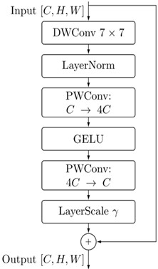
Unless otherwise stated, feature maps follow the [ $C, H, W$ ] convention. Each ConvNeXtBlock includes a depthwise 7×7 convolution for local modeling, followed by LayerNorm and two pointwise 1×1 convolutions with GELU to expand and project channels. A residual connection with learnable LayerScale stabilizes optimization. The ConvNeXt-T backbone comprises the following components:

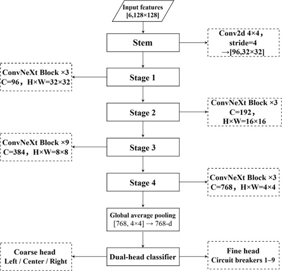
(1) Stem layer: A 4×4 convolution with stride 4 projects the six-channel input to 96 channels, while reducing the spatial resolution from 128×128 to 32×32.

(2) Four stages: each stage consists of multiple stacked ConvNeXtBlocks, with depths of (3, 3, 9, 3) and channel dimensions of (96, 192, 384, 768), respectively. Adjacent stages are connected by downsampling layers composed of a LayerNorm followed by a 2×2 convolution with stride 2, which halves the spatial resolution and doubles the number of channels. The ConvNeXtBlock module is shown in Fig. 3.

Fig. 3Schematic diagram of the ConvNeXtBlock module

(3) Global average pooling: the output of the final stage is globally pooled to obtain a 768-dimensional feature vector, which is then fed to the classifier.

(4) Training objective: inspired by weighted joint losses used in multi-task distillation [13], we optimize coarse and fine classification heads with a joint loss:

11

L = α L_{c o a r s e} + (1 - α) L_{f i n e} .

In this formulation, $α$ is selected as 0.3 via grid search, and $L_{c o a r s e}$ and $L_{f i n e}$ denote the cross-entropy losses of the coarse and fine classification heads, respectively. The coarse head provides region-level supervision with a weight of 30 %, encouraging the model to first separate the cabinet into left, middle, and right regions and thereby reducing large-offset errors (e.g., confusing breaker 1 on the far left with breaker 9 on the far right). The fine head, weighted at 70 %, then discriminates the specific breaker position within each region. Joint training encourages the model to capture both global structure and local position details.

We use the coarse head only as a training-time regularizer and discard it at inference, reporting predictions from the fine head only. In practical inspection, however, each complete recording requires a single stable decision. Since breaker operation durations vary across samples and each recording is segmented into multiple clips, we aggregate clip-level posteriors to obtain recording-level predictions. Specifically, for a recording consisting of N_F clips, let $p_{i} \in R^{9}$ denote the fine-head softmax probability vector for the i-th clip. The file-level posterior $P_{F}$ is computed by averaging: $P_{F} = \frac{1}{N_{F}} \sum_{i = 1}^{N_{F}} p_{i}$ , where NF is the number of clips in the recording. The final file-level prediction is then ${\hat{y}}_{F} = a r g {m a x}_{c} p_{F} (c)$ , which yields the predicted breaker label for the recording. File-level accuracy and Macro-F1 are computed from ${\hat{y}}_{F}$ over all recordings. This posterior-averaging strategy reduces the variance of clip-level predictions and improves robustness to variable operation durations and occasional noisy clips.

The overall ConvNeXt-T network framework is shown in Fig. 4.

Fig. 4ConvNeXt-T network framework

4. Stereo-enhanced cross-channel attention

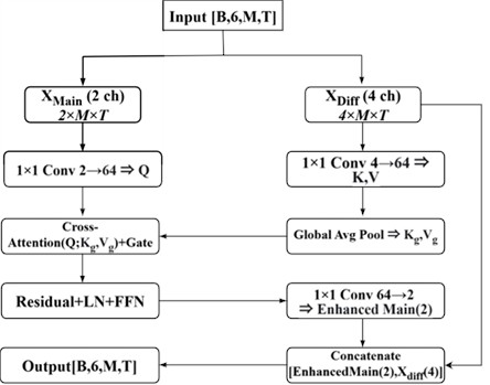
This section presents the Stereo-Enhanced Cross-Channel Attention (SECCA) module, which enhances the six-channel input before it enters ConvNeXt. SECCA treats the two content channels ( $L_{m e l}$ and $R_{m e l}$ ) as the Query source and the four spatial channels, including ILD, IPD, and GCC features, as the Key/Value sources, producing cross-channel guided attention [15] rather than conventional self-attention [17]. The design explicitly encodes the intuition that spatial cues should guide content modeling, and it is consistent with lightweight channel-gating mechanisms in CNN attention modules [18].

We organize tensors in $[B, C, M, T]$ format, where $B$ is the batch size, $C =$ 6 is the channel count, and MMM and TTT denote frequency and time. Given input $X$ , we split it into a content branch $X_{m a i n}$ with two channels and a spatial branch $X_{d i f f}$ with four channels. A 1×1 convolution maps $X_{m a i n}$ to the Query $Q$ , while two 1×1 convolutions map $X_{d i f f}$ to the Key $K$ and Value $V$ . We then apply global pooling to $K$ and $V$ to obtain compact spatial descriptors $K_{g}$ and $V_{g}$ , compute global cross-attention between $Q$ and the pooled spatial descriptors, and pass the result through a sigmoid function to form a two-channel gating vector $G$ . The gating vector $G$ is broadcast over the time-frequency plane to modulate $X_{m a i n}$ at each bin. The enhanced content features are refined with a residual connection, LayerNorm, and a lightweight feed-forward network. Finally, the enhanced two-channel content output is concatenated with $X_{d i f f}$ to restore a six-channel tensor, which is fed to ConvNeXt-T. The detailed architecture of the SECCA module is shown in Fig. 5.

Fig. 5Detailed architecture of the SECCA module

For clarity, we define the left-right swap transformation used in training and evaluation. For a feature tensor X = [L, R, ILD, IPD_cos, IPD_sin, GCC], the transformed tensor $T (X)$ is [R, L, -ILD, IPD_cos, -IPD_sin, flip_lag(GCC)]. The corresponding label permutation is $P (y) = 10 - y$ for nine positions. An exactly left-right consistent model would satisfy $f (T (X)) = P f (X)$ . The present network is not claimed to guarantee this equality by construction because the convolutional projections are learned. Instead, SECCA preserves the physically meaningful branch transformation and LR-swap augmentation encourages empirical consistency under T.

Table 1LR-swap feature transformation rule

Input channel	After LR-swap	Physical meaning
L_mel	R_mel	Left/right content channels are exchanged
R_mel	L_mel	Left/right content channels are exchanged
ILD	–ILD	Interaural level-difference sign is reversed
IPD_cos	IPD_cos	Cosine phase difference is even-symmetric and remains unchanged
IPD_sin	–IPD_sin	Sine phase difference is odd-symmetric and changes sign
GCC	flip_lag(GCC)	The GCC delay axis is mirrored
label y	$P (y) = 10 - y$	The nine breaker positions are mirrored from left to right

To validate this point, we performed an LR-swap consistency test on the holdout test set. After applying $T$ to the six-channel inputs, the file-level prediction matched the mirrored original prediction for 94.44 % of recordings; clip-level consistency was 89.66 %, and the mean KL divergence between the original posterior and the mirrored swapped posterior was 0.1515. These results support the intended stereo-consistency behavior, while avoiding the stronger claim of strict architecture-guaranteed left-right consistency.

Table 2LR-swap consistency results of ConvNeXt-T + SECCA

Metric	Value
Number of test files	180
Number of test clips	619
Original file-level accuracy	94.44 %
File-level accuracy after LR-swap with mirrored labels	91.67 %
File-level mirror-prediction consistency	94.44 %
Clip-level mirror-prediction consistency	89.66 %
Mean KL[p(original) \|\| mirror(p(swapped))]	0.1515

5. Results and analysis

5.1. Training configuration

Experiments were conducted on an NVIDIA GeForce RTX 4070 GPU (8 GB) using PyTorch 2.0. We trained models with AdamW (initial learning rate 3×10^-4, weight decay 5×10^-4) and a cosine annealing schedule (minimum learning rate 1×10^-6). The batch size was 24 and training ran for up to 100 epochs with early stopping (patience 15).

We used three-fold grouped cross-validation at the recording level to prevent data leakage: clips from the same recording never appear in both training and validation splits. Each fold uses 600 recordings for training and 300 for validation; results are reported as mean ± standard deviation of file-level metrics over the three folds.

We report accuracy, recall, and F1-score. Macro-F1 (the unweighted mean of per-class F1) is used as the primary metric to reduce sensitivity to class imbalance.

5.2. Analysis of training results

The file-level accuracy curves on fold 2 for ConvNeXt and ConvNeXt-T + SECCA are shown in Fig. 6.

Fig. 6Comparison of file-level accuracy between the baseline and the SECCA module

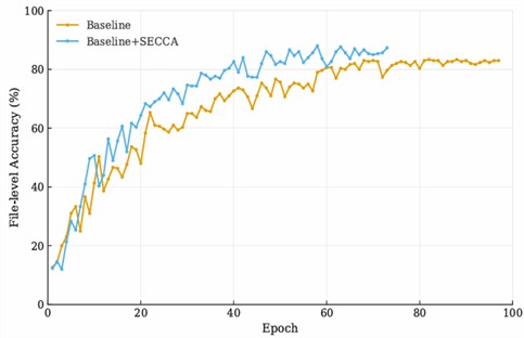
Fig. 6 shows that ConvNeXt-T + SECCA consistently achieves higher file-level accuracy and converges in fewer epochs than the baseline. With identical hyperparameters and early-stopping criteria, the SECCA model peaks at 88.0 % (epoch 58) whereas the baseline peaks at 83.33 % (epoch 82), indicating improved generalization rather than a trivial gain from additional parameters.

Table 3 reports file-level per-position accuracy for the baseline and SECCA-enhanced models, defined as the fraction of recordings (files) from each position that are correctly classified.

As summarized in Table 3, SECCA improves accuracy at most positions.

Table 3Comparison of accuracy at each breaker position

Position	ConvNeXt accuracy (%)	+SECCA accuracy (%)
1	87.5	90.0
2	66.7	86.7
3	93.3	86.7
4	82.5	87.5
5	86.7	93.3
6	83.3	76.7
7	87.5	92.5
8	93.3	93.3
9	83.3	93.3

The largest gains occur at positions 2 and 9: accuracy increases from 66.7 % to 86.7 % at position 2 and from 83.3 % to 93.3 % at position 9, suggesting that SECCA reduces confusion between adjacent breakers. Positions 4, 5, and 7 also improve from 82.5 %, 86.7 %, and 87.5 % to 87.5 %, 93.3 %, and 92.5 %, respectively.

The decreases at positions 3 and 6 should also be noted. In Table 3, position 3 drops from 93.3 % to 86.7 %, and position 6 drops from 83.3 % to 76.7 %. Each 6.7-point decrease corresponds to two additional errors out of 30 validation recordings. Inspection of the misclassified files shows that these errors are concentrated in adjacent-position confusions, mainly 3→2/4 and 6→5/7, with no large-offset mislocalization. This behavior is consistent with the physical layout: positions 3 and 6 lie near transition regions where neighboring cabinet responses have similar ILD, IPD, and GCC patterns under the fixed recorder geometry. SECCA improves the global average by emphasizing spatial cues, but in these boundary cases the same cues can become ambiguous. This limitation motivates future data collection with additional recorder placements and more samples around the affected positions.

Fig. 7 visualizes predicted versus true positions for 300 validation samples in fold 2. Predictions largely follow the stepwise ground-truth curve: most errors are within one adjacent position and only two samples deviate by two positions. No larger deviations were observed, indicating that the proposed model reliably locks onto the correct breaker in most cases.

Fig. 7Analysis of position offsets for predicted circuit-breaker locations

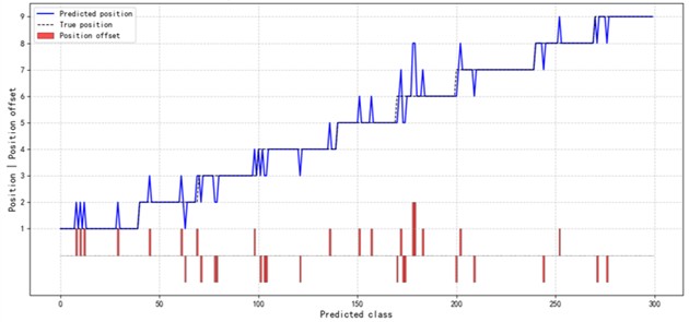
Table 4 reports the mean and standard deviation of file-level Macro-F1 under three-fold cross-validation for ConvNeXt-T and ConvNeXt-T + SECCA.

Adding SECCA improves file-level Macro-F1 to 84.79 %±2.26 % (+4.10 points over ConvNeXt-T), as shown in Table 4. File-level accuracy increases from 81.0 % to 84.9 %, and the best single-fold accuracy reaches 88.0 %. These results indicate that spatially guided cross-channel attention improves generalization at the recording level.

Misclassification analysis: to better understand how SECCA improves localization, we inspected representative recordings that are corrected by SECCA as well as cases where SECCA introduces new errors (Table 5).

Table 5 shows that corrections are concentrated in confusions between neighboring positions, with notable improvements for closing sounds under high current (315 A and 630 A). For example, “Position2_315A_closing_01” is misclassified as position 3 by the baseline but corrected to position 2 by SECCA, consistent with stronger guidance from IPD and GCC cues. Across three-fold cross-validation, SECCA corrects approximately 90 such misclassifications.

Table 4Comparison of file-level F1-scores between the baseline and SECCA

Method	File-level F1-score	F1 improvement
ConvNeXt	80.69±1.48
ConvNeXt-T + SECCA	84.79±2.26	+4.10

Table 5Typical cases corrected by SECCA

File ID	Position	ConvNeXt prediction	+SECCA prediction
Successfully corrected cases (partial)
Position2_315A_closing_01	2	3	2
Position2_315A_closing_04	2	3	2
Position7_315A_closing_01	7	8	7
Position8_315A_closing_02	8	9	8

5.3. Comparison with classical dual-microphone baselines and complexity

To address whether a conventional dual-microphone localization method is sufficient for this task, we added a unified holdout comparison using the same dataset split. For a two-microphone linear recorder, delay-and-sum beamforming effectively reduces to scanning candidate inter-channel delays; therefore, the GCC-PHAT + TDOA peak baseline serves as the classical time-delay/beamforming reference. We also tested GCC-PHAT features with SVM, ILD/IPD statistics with SVM, and all handcrafted stereo features with SVM or Random Forest classifiers.

Table 6Comparison of classical methods, ConvNeXt-T baseline, and the proposed method

Method	Type	File Acc. (%)	File Macro-F1 (%)
ILD/IPD + SVM	Handcrafted stereo statistics	11.11	11.38
GCC-PHAT + TDOA peak	Classical time-delay localization	23.33	18.26
GCC-PHAT + SVM	GCC feature + classifier	36.67	36.24
All handcrafted features + SVM	ILD/IPD/GCC/TDOA + classifier	40.56	40.59
All handcrafted features + Random Forest	Traditional feature-engineering upper baseline	47.22	45.88
ConvNeXt-T baseline	Deep learning baseline	93.33	93.33
ConvNeXt-T + SECCA	Proposed method	94.44	94.48

Table 6 shows that classical time-delay and handcrafted-feature methods are insufficient for the nine-position near-field cabinet task. GCC-PHAT + TDOA peak detection obtains only 23.33 % file-level accuracy, and the best handcrafted-feature baseline reaches 47.22 %. In contrast, the ConvNeXt-T baseline already reaches 93.33 %, and adding SECCA further improves the holdout file-level accuracy to 94.44 %. The results indicate that the main difficulty is not only estimating a single inter-channel delay, but also modeling the coupled time-frequency content and stereo spatial cues of transient breaker sounds.

The complexity measurements in Table 7 were obtained on an NVIDIA RTX 4070 GPU. SECCA adds only 0.067M parameters to ConvNeXt-T, increasing the parameter count by about 0.24 %. The single-clip latency increases from 6.09 ms to 7.31 ms, which remains compatible with online inspection because one complete recording contains only a small number of 2-s clips and file-level aggregation is performed after clip inference. More complex CRNN- and TF-GridNet-style baselines are relevant to broader audio localization and multi-source scenes, but their objectives and deployment costs are not directly matched to the single-event fixed-recorder cabinet setting; they are therefore treated as future same-protocol baselines rather than as direct baselines in this study.

Table 7Complexity comparison of ConvNeXt-T and SECCA for an input size of 1×6×128×128

Model	Parameters (M)	MACs (G)	Latency (ms/clip)
ConvNeXt-T baseline	27.834	1.459	6.09 ± 1.02
ConvNeXt-T + SECCA	27.901	2.283	7.31 ± 1.28
ConvNeXt-T + CBAM + SECCA	28.000	2.283	8.73 ± 1.35

5.4. Noise robustness and current deployment scope

We further tested feature-domain Gaussian perturbations on the holdout set using the same posterior averaging strategy as the main evaluation. This experiment does not replace raw acoustic validation under every field-noise condition, but it provides a controlled sensitivity check for the six-channel input representation.

Table 8File-level accuracy under feature-domain Gaussian perturbations

Noise sigma	0.0	0.2	0.4	0.6	0.8	1.0
File Acc. (%)	94.44	95.56	95.00	93.33	90.56	90.00

As shown in Table 8, accuracy remains above 93 % for sigma ≤ 0.6 and remains 90.00 % even at sigma = 1.0. The model therefore shows moderate robustness to severe feature perturbation. Nevertheless, the current dataset contains one fixed recorder placement and single-breaker operations only. Simultaneous multiple breaker operations, large sensor displacement, microphone aging, channel imbalance, and long-term sensor degradation were not directly measured in this study. These factors are now treated as explicit limitations and will require additional field data and multi-source modeling in future work.

5.5. Attention visualization analysis

To better understand the role of the SECCA module in stereo sound source localization, we conducted both visualization and statistical analysis of its attention responses on the test set. The results reveal a clear frequency-selective pattern, with higher attention in the low- and high-frequency regions and relatively lower attention in the mid-frequency region. On the time-frequency plane, SECCA also focuses on temporally and spectrally informative regions associated with breaker operations, suggesting that it adaptively emphasizes spatially discriminative cues rather than uniformly enhancing all features.

Fig. 8Frequency-domain attention response of the SECCA module

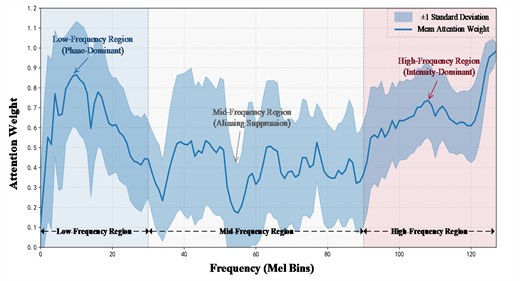
To further examine this behavior, we extracted the attention gating maps of SECCA and summarized them across the test set. For each sample, the attention weights were first averaged over time and then aggregated across samples for each Mel band. As shown in Fig. 8, where the solid line and shaded area denote the mean and standard deviation, respectively, SECCA exhibits a clear U-shaped frequency response. Specifically, higher attention in the low-frequency region indicates greater reliance on stable spatial cues, such as inter-channel phase and time-delay differences, for direction discrimination. The reduced attention in the mid-frequency region suggests a smaller contribution to localization, likely because this band is more susceptible to continuous hum and background noise. In the high-frequency region, attention increases again, implying that the model further exploits inter-channel energy differences that are informative for spatial discrimination. Overall, these results show that SECCA learns a frequency-selective enhancement pattern that is well aligned with the localization task.

To further illustrate this pattern, Fig. 9 presents the attention map for a representative test sample. SECCA selectively emphasizes time-frequency regions with stronger spatial cues rather than uniformly highlighting the entire operation interval. Higher responses are observed in frames with more pronounced inter-channel differences, where spatially discriminative information is more concentrated, whereas noisy or weakly discriminative regions are suppressed. Consistent with Fig. 8, attention is stronger in the low- and high-frequency regions and weaker in the mid-frequency region, indicating that SECCA enhances localization by focusing on spatially informative cues while reducing the influence of less relevant acoustic components.

Fig. 9Time-frequency attention response of the SECCA module

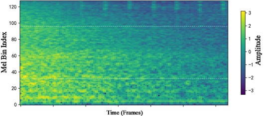
a) Original input mel spectogram

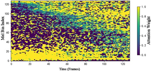
b) SECCA attention weight map

6. Conclusions

In this work, we developed a stereo-enhanced cross-channel attention framework for localizing circuit breaker operation sounds in distribution cabinets using only a fixed dual-microphone recorder. The framework combines left/right log-Mel spectrograms, ILD, IPD, and GCC-based time-delay cues in a six-channel representation, and uses the SECCA module to inject spatial information into content modeling. Evaluated on a 10-kV switchgear dataset with nine positions, two operation types, and five current levels, ConvNeXt-T + SECCA achieved a file-level Macro-F1 of 84.79 % ± 2.26 % and a file-level accuracy of 84.9 %, with a best result of 88.0 % in grouped validation. Additional holdout experiments showed 94.44% file-level accuracy against classical GCC-PHAT/TDOA and handcrafted-feature baselines. Attention visualization and LR-swap consistency analysis indicate that SECCA improves localization by adaptively emphasizing stereo spatial cues rather than by simply increasing parameter count.

Across positions, accuracy ranged from 76.7 % to 93.3 %, and most positions improved by 5-20 points over the baseline. The remaining errors were concentrated mainly between adjacent breakers, consistent with the physical layout of closely spaced cabinets. The present study is therefore best interpreted as validation under a controlled fixed-recorder deployment. Future work will extend the dataset to multiple recorder placements, simultaneous operations, and sensor-degradation conditions.

References

V. H. Coria, S. Maximov, F. Rivas-Dávalos, C. L. Melchor, and J. L. Guardado, “Analytical method for optimization of maintenance policy based on available system failure data,” Reliability Engineering and System Safety, Vol. 135, pp. 55–63, 2014, https://doi.org/10.1016/j.ress.2014.11.003

Publisher
C. Hu, “Mechanical fault diagnosis of high-voltage circuit breakers based on vibration signals,” (in Chinese), Modern Manufacturing Technology and Equipment, Vol. 61, No. 7, pp. 94–96, 2025, https://doi.org/10.16107/j.cnki.mmte.2025.0491

Publisher
M. Wu, “Automatic fault diagnosis of high-voltage vacuum circuit breakers based on abnormal current signals,” Automation Application, Vol. 65, No. 15, pp. 255–257, 2024.

Search CrossRef
Y. G. Guan et al., “A review of mechanical fault diagnosis methods for high-voltage circuit breakers,” (in Chinese), High Voltage Apparatus, Vol. 54, No. 7, pp. 10–19, 2018, https://doi.org/10.13296/j.1001-1609.hva.2018.07.002

Publisher
F. Duan et al., “Acoustic fingerprint-based mechanical fault recognition method for 10 kV high-voltage circuit breakers using fused features and residual neural networks,” (in Chinese), High Voltage Apparatus, Vol. 61, No. 3, pp. 205–213, 2025, https://doi.org/10.13296/j.1001-1609.hva.2025.03.025

Publisher
X. F. Xia et al., “Mechanical fault diagnosis method for high-voltage circuit breakers based on acoustic fingerprint analysis,” (in Chinese), High Voltage Apparatus, Vol. 57, No. 10, pp. 66–76, 2021, https://doi.org/10.13296/j.1001-1609.hva.2021.10.009

Publisher
L. J. Zhang, M. Wang, and L. Y. Luo, “Street environmental sound event detection method based on improved log-Mel spectral features,” (in Chinese), Journal of Guilin University of Electronic Technology, Vol. 40, No. 5, pp. 411–417, 2020, https://doi.org/10.16725/j.cnki.cn45-1351/tn.2020.05.007

Publisher
R. Gu, S.-X. Zhang, Y. Zou, and D. Yu, “Complex neural spatial filter: enhancing multi-channel target speech separation in complex domain,” IEEE Signal Processing Letters, Vol. 28, pp. 1370–1374, Apr. 2021, https://doi.org/10.1109/lsp.2021.3076374

Publisher
D. A. Krause and A. Mesaros, “Binaural signal representations for joint sound event detection and acoustic scene classification,” in 2022 30th European Signal Processing Conference (EUSIPCO), pp. 399–403, 2022, https://doi.org/10.23919/eusipco55093.2022.9909581

Publisher
H.-M. Jo, T.-W. Kim, and K.-C. Kwak, “Sound source localization using deep learning for human-robot interaction under intelligent robot environments,” Electronics, Vol. 14, No. 5, p. 1043, 2025, https://doi.org/10.3390/electronics14051043

Publisher
H. Y. Tang, Z. W. Chen, and W. Huang, “Analysis of GCC time-delay estimation algorithms based on microphone arrays,” (in Chinese), Computer Systems and Applications, Vol. 28, No. 12, pp. 140–145, 2019, https://doi.org/10.15888/j.cnki.csa.007173

Publisher
K. L. Wan et al., “Transformer core looseness fault diagnosis method based on Mel-GADF and ConvNeXt-T,” (in Chinese), Electric Power Automation Equipment, Vol. 44, No. 3, pp. 217–224, 2024, https://doi.org/10.16081/j.epae.202307003

Publisher
Z. X. Gao et al., “Intent recognition and slot filling based on multi-task distillation,” (in Chinese), Journal of Shaanxi Normal University (Natural Science Edition), Vol. 52, No. 3, pp. 96–104, 2024, https://doi.org/10.15983/j.cnki.jsnu.2024013

Publisher
X. Z. Zhang, Z. Y. Tan, and Y. J. Wang, “SAR image target recognition based on multi-feature and multi-representation fusion,” Journal of Radars, Vol. 6, No. 5, pp. 492–502, 2017.

Search CrossRef
F. Hu, X. Song, R. He, and Y. Yu, “Sound source localization based on residual network and channel attention module,” Scientific Reports, Vol. 13, No. 1, Apr. 2023, https://doi.org/10.1038/s41598-023-32657-7

Publisher
Z. Liu, H. Mao, C.-Y. Wu, C. Feichtenhofer, T. Darrell, and S. Xie, “A ConvNet for the 2020s,” in IEEE/CVF Conference on Computer Vision and Pattern Recognition (CVPR), pp. 11966–11976, 2022, https://doi.org/10.1109/cvpr52688.2022.01167

Publisher
A. Vaswani et al., “Attention is all you need,” in Advances in Neural Information Processing Systems, 2017.

Search CrossRef
J. Hu, L. Shen, and G. Sun, “Squeeze-and-Excitation Networks,” in IEEE/CVF Conference on Computer Vision and Pattern Recognition, pp. 7132–7141, 2018, https://doi.org/10.1109/cvpr.2018.00745

Publisher
S. Adavanne, A. Politis, J. Nikunen, and T. Virtanen, “Sound event localization and detection of overlapping sources using convolutional recurrent neural networks,” IEEE Journal of Selected Topics in Signal Processing, Vol. 13, No. 1, pp. 34–48, Mar. 2018, https://doi.org/10.1109/jstsp.2018.2885636

Publisher
D. Salvati, C. Drioli, and G. L. Foresti, “Time delay estimation for speaker localization using CNN-based parametrized GCC-PHAT features,” in Interspeech 2021, pp. 1479–1483, 2021, https://doi.org/10.21437/interspeech.2021-988

Publisher
M. Cobos, F. Antonacci, L. Comanducci, and A. Sarti, “Frequency-sliding generalized cross-correlation: a sub-band time delay estimation approach,” IEEE/ACM Transactions on Audio, Speech, and Language Processing, Vol. 28, pp. 1270–1281, 2020, https://doi.org/10.1109/taslp.2020.2983589

Publisher

About this article

Received

March 4, 2026

Accepted

June 23, 2026

Published

August 3, 2026

SUBJECTS

Acoustics, noise control and engineering applications

DOI

https://doi.org/10.21595/jve.2026.26265

Keywords

circuit breaker

sound source localization

stereo audio

cross-channel attention

deep learning

Acknowledgements

The authors have not disclosed any funding.

Data Availability

The datasets generated during and/or analyzed during the current study are available from the corresponding author on reasonable request.

Author Contributions

Guangmin Gu and Wei Zhang performed the measurements. Fei Wan and Like Zhao contributed to the study planning and supervised the work. Guangmin Gu processed the experimental data, carried out the analysis, drafted the manuscript, and designed the figures. Like Zhao contributed to the interpretation of the results and revised the manuscript. All authors discussed the results and approved the final manuscript.

Conflict of interest

The authors declare that they have no conflict of interest.

This is an open access article distributed under the Creative Commons Attribution License, which permits unrestricted use, distribution, and reproduction in any medium, provided the original work is properly cited.

G. Gu, W. Zhang, F. Wan, and L. Zhao, “Circuit breaker sound source localization method based on cross-channel attention fusion,” Journal of Vibroengineering, Vol. 28, No. 6, –15, Aug. 2026, https://doi.org/10.21595/jve.2026.26265

Copy Extrica

Copied to clipboard!

TY  - JOUR
DO  - 10.21595/jve.2026.26265
UR  - https://doi.org/10.21595/jve.2026.26265
TI  - Circuit breaker sound source localization method based on cross-channel attention fusion
T2  - Journal of Vibroengineering
AU  - Gu, Guangmin
AU  - Zhang, Wei
AU  - Wan, Fei
AU  - Zhao, Like
PY  - 2026
DA  - 2026/08/03
PB  - Extrica
VL  - 28
IS  - 6
SN  - 1392-8716
SN  - 2538-8460
ER  - 

Copy Ris

Copied to clipboard!

@article{doi_10.21595/jve.2026.26265,
  title = {Circuit breaker sound source localization method based on cross-channel attention fusion},
  author = {Gu, Guangmin and Zhang, Wei and Wan, Fei and Zhao, Like},
  journal = {Journal of Vibroengineering},
  year = {2026},
  month = {8},
  volume = {28},
  number = {6},
  doi = {10.21595/jve.2026.26265},
  url = {https://doi.org/10.21595/jve.2026.26265},
  publisher = {Extrica},
  issn = {1392-8716},
  eissn = {2538-8460},
}

Copy Bibtex

Copied to clipboard!

[1]G. Gu, W. Zhang, F. Wan, and L. Zhao, “Circuit breaker sound source localization method based on cross-channel attention fusion,” Journal of Vibroengineering, Aug. 2026, doi: 10.21595/jve.2026.26265.

Copy IEEE

Copied to clipboard!

Gu, Guangmin, Wei Zhang, Fei Wan, and Like Zhao. “Circuit breaker sound source localization method based on cross-channel attention fusion.” Journal of Vibroengineering 28, no. 6 (2026). https://doi.org/10.21595/jve.2026.26265.

Copy Chicago

Copied to clipboard!

Circuit breaker sound source localization method based on cross-channel attention fusion

Abstract

1. Introduction

2. Audio data acquisition and acoustic modeling

2.1. Experimental setup and procedure

2.2. Feature extraction method for circuit-breaker acoustic fingerprints

2.3. Stereo acoustic fingerprint feature extraction

3. ConvNeXt-T network

4. Stereo-enhanced cross-channel attention

5. Results and analysis

5.1. Training configuration

5.2. Analysis of training results

5.3. Comparison with classical dual-microphone baselines and complexity

5.4. Noise robustness and current deployment scope

5.5. Attention visualization analysis

6. Conclusions

References

About this article

Related Articles