Error mechanisms and applicability boundaries of the vibration input method in tunnel seismic response analysis

Tan, Xukai; Chen, Zhengdong; Yuan, Jiamu; Lu, Guangping; Gao, Feng; Ding, Hao

doi:10.21595/jve.2026.25948

Journal of Vibroengineering

Browse Journal

Submit article

Published: August 19, 2026

Check for updates

Error mechanisms and applicability boundaries of the vibration input method in tunnel seismic response analysis

Xukai Tan¹

Zhengdong Chen²

Jiamu Yuan³

Guangping Lu⁴

Feng Gao⁵

Hao Ding⁶

^{1, 4, 5}State Key Laboratory of' Mountain Bridge and Tunnel Engineering, Chongqing Jiaotong University, Chongqing, China

^{2, 3, 1, 5}School of Civil Engineering, Chongqing Jiaotong University, Chongqing, China

^{6, 1}China Merchants Chongqing Communications Technology Research and Design Institute Co., Ltd, Chongqing, China

Corresponding Author:

Xukai Tan

Cite the article Download PDF

Article in Press

Downloads 60

Abstract

This study evaluates the applicability of traditional vibration input methods in tunnel seismic analysis to address limited calculation accuracy and ambiguous applicability. The vibration input method, wave input method, and theoretical solutions are compared to clarify the error mechanism and main influencing factors. Through correlation analyses, the relationships between model dimensions, geological parameters, and accuracy are established. Then an innovative approach is proposed to improve the calculation accuracy and refine the scope of applicability. The results indicate that the assumed bedrock surface position and model boundaries can significantly affect the accuracy of the model, with the height and wave velocity of the surrounding rock being key control parameters. When the model height is fixed, the correlation coefficient between vibration and wave input results shows three stages of change with increasing width: rapid increase, deceleration growth, and asymptotic convergence to 1. In the case of a fixed width, as the height increases, the coefficient follows a trend of “approximately stable slightly decreasing”. The optimal aspect ratio is 1:2. Size optimization formulas under different rock conditions and methods for selecting analysis time periods are proposed to clarify the engineering applicability of the vibration input method.

Error mechanisms and applicability boundaries of the vibration input method in tunnel seismic response analysis

Highlights

This study reveals that the vibration input method's inferior accuracy stems from two error mechanisms: side boundary–structure coupling and bottom boundary standing waves, clarifying the inherent limitations of traditional applicability assumptions.
Quantitative geometry–fidelity relationships are established: the correlation with wave input shows a three-stage trend with width and a near-stable decline with height. The optimal aspect ratio is 1:2, with boundary-to-tunnel distance ≥6× the span.
A practical three-step methodology is proposed: (i) increase model height to delay reflected waves; (ii) adopt a 1:2 aspect ratio; (iii) identify the effective time window via 1D wave theory—enabling confident use of this efficient method.

1. Introduction

As a key component of lifeline infrastructure, tunnels are essential for seismic safety. The seismic response of tunnels is controlled by complex soil-structure interaction mechanisms [1]. The construction of resilience curves depends heavily on the computational accuracy of structural seismic responses [2]. In numerical simulations of tunnel seismic response, selecting an appropriate ground motion input method is crucial for accurate results. Although the traditional viscous boundary input method is convenience and simple, its calculation accuracy is relatively low and its applicability is limited. In addition, there is a lack of clear standards to define its scope of application. Therefore, the study of the applicability and calculation accuracy of the viscous boundary input method in tunnel seismic analysis has significant theoretical and practical significance. It also has direct implications for promoting seismic design standards and ensuring engineering safety.

In seismic response analysis of tunnels, the selection of seismic input method is critical for the accuracy of numerical simulations. There are two commonly used methods: the wave input method, and the vibration input method. The wave input method can accurately simulate wave propagation and scattering by applying seismic motion through equivalent nodal forces. This method is particularly suitable for complex geological environments and scenes involving oblique wave incidence [3-5]. It has been demonstrated that viscoelastic artificial boundaries can provide stable results [6-8]. However, this method involves complex preprocessing procedures and high computational requirements. In addition, accurately determining the equivalent nodal force requires accurate identification of wavefield characteristics [9]. In contrast, the vibration input method directly specifies the displacement or acceleration time history in the model. However, it is only effective when dealing with rigid bedrock or uniform displacement boundary conditions [10-12]. Displacement-based vibration input may lead to significant inaccuracy (such as tunnel displacement responses as low as 0.12 of the value obtained using nodal force input). Meanwhile, due to the reflection of stray waves at the boundary, acceleration-based input is susceptible to numerical instability [13-14]. Therefore, the vibration input method is only suitable for relatively simple sites (such as flat ground and vertically propagating seismic waves). In cases involving steep slopes, tunnel entrances, or heterogeneous formations, it fails to fully consider spatial variability and traveling wave effects [15].

The improvement in the vibration input method has focused on optimizing boundary conditions and adjusting input mechanisms. Examples include using layered acceleration input to explain the temporal variation of wave propagation and combing uniform displacement boundaries with viscoelastic boundaries and substructure techniques to reduce artificial wave reflections [16]. However, this method is still limited by its inability to explain multi wave reflection and scattering effects, which poses ongoing challenges for its application in complex seismic environments.

Previous research mainly focused on comparing the results of vibration input method and wave input method in tunnel seismic analysis. However, there is still a clear lack of systematic theoretical explanation to the relationship between these two methods and the physical mechanisms in their differences. More specifically, two critical issues remain unresolved: (1) quantitative decomposition of the total error to the vibration input method; (2) quantitative definition of its scope of application. Solving these fundamental problems is a prerequisite for fully utilizing the computational efficiency advantage of vibration input method in numerical simulation of tunnel seismic response.

This study compares and analyzes the vibration input method and wave input method, as well as the factors influencing these differences using a free-field model. Correlation and sensitivity analysis are used to systematically examine the impact of model size, geological parameters, and assumptions about bedrock interfaces on the accuracy of vibration input methods. This study proposes key technical strategies to improve the accuracy of the vibration input method and scientifically delineate its scope of applicability.

2. Implementation methods and a comparative analysis of wave input method and vibration input method

2.1. Implementation of the wave input method

Based on wave theory, this method transforms physical problems in infinite domains into numerically solvable models in finite domains through rigorous mathematical formulas. The main principle of this method is to transform the wave propagation problem in unbounded regions into finite field simulation by introducing artificial boundaries and equivalent node forces. The procedure includes:

(1) Governing equation of wave motion: The propagation of waves in a medium is governed by scalar wave equations:

1

\frac{\partial^{2} u}{\partial t^{2}} = c^{2} \nabla^{2} u,

where: $u (r, t)$ denotes the wave function; $c$ represents the wave velocity, and $\nabla^{2}$ is the Laplace operator.

According to the principle of linear superposition, the total wave field can be decomposed into a free field and a scattered field. A free field corresponds to the propagation of seismic waves through undisturbed natural geological formations. On the other hand, the scattering field constitutes additional wave components caused by disturbances in the original wavefield. This scattering component originates from the structural interface and propagates infinitely outward.

(2) Transformation from an infinite to a finite domain and artificial boundaries.

In numerical simulation, modeling an infinite domain directly is infeasible. To address this issue, a viscoelastic artificial boundary is introduced to truncate the domain and define a finite calculation region. Under this artificial boundary, the combined effect of the input force caused by free-field stress and the compensating force provided by the viscoelastic boundary ensures that the numerical solution within the calculation domain satisfies the governing wave equation. In this numerical model, both the bottom and lateral boundaries are treated as viscoelastic artificial boundaries. The governing equation is expressed as follows:

2

F_{b} = A_{b} (K u_{b}^{i} + C {\dot{u}}_{b}^{i} + σ_{b}^{i}),

where: $F_{b}$ denotes the equivalent load at the boundary node; $A_{b}$ represents the equivalent nodal area; $K$ and $C$ are the stiffness and damping coefficients of the boundary spring, respectively. These coefficients depend on the shear modulus $G$ , density $ρ$ , wave velocity (either P-wave velocity $c_{p}$ or S-wave velocity $c_{s}$ ), and boundary correction coefficients (normal direction $α_{N}$ , tangential direction $α_{T}$ ; $u_{b}^{i}$ , ${\dot{u}}_{b}^{i}$ and $σ_{b}^{i}$ refer to the free-field displacement, velocity, and stress, respectively.

(3) Governing equations of the finite domain model.

In the seismic response analysis of tunnels, the wave input formulation for the finite domain model is mainly based on a viscoelastic artificial boundary. The equivalent nodal force method is combined to achieve seismic motion input. The governing equations are expressed as follows:

3

M \ddot{u} + C \dot{u} + K u = F_{b},

where: $M$ , $C$ and $K$ denote the global mass, damping, and stiffness matrices of the system, respectively; $u$ , $\dot{u}$ and $\ddot{u}$ represent the displacement, velocity and acceleration vectors, respectively; and $F_{b}$ refers to the seismic load vector using the equivalent nodal force method.

2.2. Implementation of the vibration input method

Based on d'Alembert’s principle, the vibration input method is used to analyze the seismic response of tunnels. Assuming there is a bedrock interface, seismic excitation will be transformed into inertial forces applied throughout the entire model. This methodology avoids directly inputting seismic waves. Instead, equivalent loads are applied, and the analysis emphasizes the governing of relative displacement of internal structural forces. In the numerical model, fixed constraints are applied to the bottom boundary, and viscoelastic artificial boundaries are applied to the side boundaries. The core governing equation for the solution is expressed as follows:

4

M {\ddot{u}}^{'} + C {\dot{u}}^{'} + K u^{'} = - M {\ddot{u}}_{g},

where: $M$ , $C$ and $K$ denote the global mass matrix, global damping matrix, and global stiffness matrix of the system, respectively; $u$ , $\dot{u}$ and $\ddot{u}$ represent the relative displacement vector, relative velocity vector, and relative acceleration vector of the system relative to the bedrock surface, respectively; ${\ddot{u}}_{g}$ at the input acceleration at the bedrock surface.

2.3. Comparative analysis of vibration and wave input methods

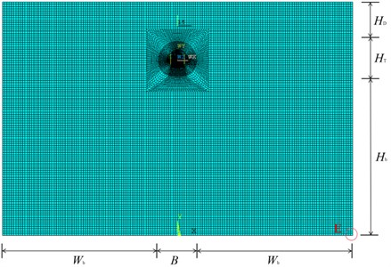
A free-field soil model is established based on the standard cross-sectional dimensions of a double-track tunnel. To ensure sufficient spatial discretization accuracy for dynamic analysis, the finite element standard proposed by Kuhlemeyer et al. [17] is strictly followed, which stipulates that the maximum element size should not exceed one tenth of the shear wavelength of seismic waves. The input pulse wave has a frequency of 4 Hz, and the shear wave velocity of the site ranges from 200 to 600 m/s, corresponding to a shear wavelength of 50 to 150 m. Consequently, the maximum permissible element size is 5 m. In actual meshing, the entire model adopts a mapping mesh strategy, with an element size from 0.5 m to1.0 m. This discretization scheme strictly meets the above accuracy requirements and ensures faithful capture of wave propagation characteristics. The detailed model dimension parameters are expressed as in Eq. (5) and Eq. (6). Fig. 1(a) shows the geometric configuration of the model, where point E indicates a representative boundary reference location:

5

H_{t o t a l} = H_{D} + H_{T} + H_{b},

6

W_{t o t a l} = B + 2 W_{b},

where: $H_{t o t a l}$ and $W_{t o t a l}$ denote the overall height and width of the model, respectively. $H_{D}$ corresponds to the tunnel burial depth, taken as 20 ml. $H_{T}$ indicates the tunnel height, taken as 12 m. $H_{b}$ refers to the vertical distance from the bottom boundary of the model to the tunnel invert, taken as 72 m. $B$ represents the tunnel span, taken as 12 m. $W_{b}$ defines the horizontal distance from the side boundary of the model to the tunnel sidewall, with a value of 72 m.

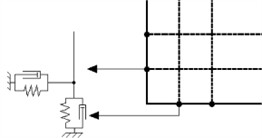
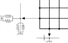
In the wave input method model, both the bottom and lateral boundaries use viscous-spring artificial boundaries, as shown in Fig. 1(b). In contrast, the bottom boundary is fixed in the inertial input method model, and viscous-spring artificial boundaries are applied to the lateral boundaries, as shown in Fig. 1(c).

Fig. 1Schematic diagram of the finite element model: a) finite element model; b) boundary conditions of the wave input method model; and c) boundary conditions of the vibration input method model

Schematic diagram of the finite element model: a) finite element model; b) boundary conditions of the wave input method model; and c) boundary conditions of the vibration input method model

a)

b)

c)

The surrounding rock and soil layers are designed as Grade VI. The material parameters are set as: elastic modulus $E =$ 100 MPa, Poisson’s ratio $υ =$ 0.3, and density $ρ =$ 1700 kg/m³. Based on the theory of elasticity, the shear wave velocity of the rock-soil medium is calculated as $v_{s} =$ 150.4 m/s.

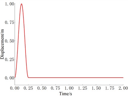
Dynamic excitation is applied as a vertically incident, horizontal, unit-impulse shear-displacement wave. Eq. (7) shows its mathematical representation, and Fig. 2 shows the waveform. In the wave input method, the equivalent nodal forces for the lateral and bottom boundaries are calculated using Eq. (2) and applied to the boundary nodes. In the vibration input method, the acceleration time history is obtained by taking the second-order time derivative of Eq. (4), and this signal is applied as the input load across the entire model:

7

u (t) = \frac{1}{2} [1 - \cos (8 π f t)],

where: $f =$ 4.0, 0 $\leq t \leq$ 0.25.

Fig. 2Unit impulse shear displacement wave

To compare the calculation results under different earthquake input methods, three key areas: the top of the model (A), the tunnel arch top (B), and the bottom boundary (C), are selected for analysis. To verify the fundamental wave propagation behavior of the numerical model without tunnel structure, the theoretical solution to the one-dimensional wave equation is introduced as a benchmark. The general solution based on d'Alembert’s formula is given as:

8

u (y, t) = f (y - c t) + g (y + c t),

where $f (y - c t)$ denotes a wave propagating in the positive $y$ -direction (upward); $g (y + c t)$ represents a wave propagating in the negative $y$ -direction (downward), and $c$ is the shear-wave velocity of the medium. This formulation indicates that the displacement field $u (y, t)$ at any arbitrary location in the free field is governed by the superposition of two counter-propagating wave components. Therefore, it provides a theoretical basis for subsequent wavefield decomposition and identification of the arrival time of reflected waves.

Fig. 3 compares the displacement results of the wave motion input method and one-dimensional wave theory solution. As shown in Fig. 3, the displacement responses at points A, B, and C using the wave input method are consistent with the one-dimensional wave theory solution. This method accurately simulates the full propagation process of seismic waves. It includes the incidence of pulse waves from the bottom boundary, their reflection at the top free surface, and the physical phenomenon where the incident and reflected waves overlap at the surface, resulting in amplitude doubling. Eventually, the waves are absorbed and transmitted through the bottom boundary. Therefore, the calculation results obtained from the wave input method are adopted as the benchmark to evaluate the accuracy of the vibration input method. Fig. 4 compares the stress responses at point B (the tunnel vault) between the vibration and wave input methods.

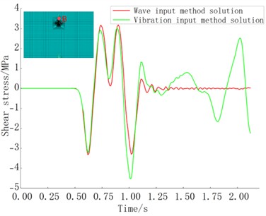
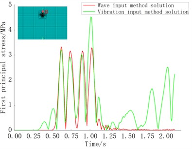
A pulse wave is applied at point B at the time interval of 0.54-1.08 s, as shown in Fig. 4. 1) The time-history responses of shear stress and the first principal stress obtained by the vibration and wave input methods have a high consistency at $T <$ 1.08 s. The fluctuations of the two methods are basically the same, mainly with slight differences in oscillation amplitude. 2) The response characteristics are different significantly after1.08 s. The wave input method introduces a viscoelastic boundary at the bottom, effectively absorbing incident wave energy. Therefore, the waves propagating in the formation gradually attenuate and disappear, causing the response to decay to zero. In contrast, the vibration input method models the bottom boundary as a fully fixed constraint that lacks energy absorption capacity. The seismic waves that encounter this boundary are completely reflected and re-enter the formation, producing a standing wave effect. This phenomenon induces persistent and significant responses at observation points in subsequent time intervals. This causes sustained and significant reactions at the observation point in subsequent time intervals.

Fig. 3Comparison between the wave input method solution and the theoretical solution

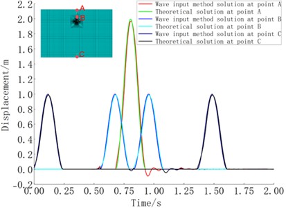
Fig. 4Comparison between the vibration input method solution and the wave input method solution: a) shear stress; and b) first principal stress

a)

b)

Comprehensive analysis shows that the vibration input method is not as accurate as the wave input method in simulating tunnel seismic analysis. First, in the absence of basic boundary reflection, the vibration input method has accurate deviations. Analysis suggests that these errors mainly caused by the coupling effect between the model dimensional scale and the structural natural vibration; Second, when using the vibration input method, the standing wave effect caused by base boundary reflections exacerbates calculation inaccuracy. This is closely related to the simplified assumption of the bedrock surface. Therefore, this study examines the mechanisms and patterns behind these two types of errors.

3. Sensitivity analysis of the accuracy of the vibration input method with respect to various influencing factors

In this study, the results of the wave-based input method are used as the benchmark. Using the Pearson correlation coefficient as a statistical indicator, the consistency between the results of the vibration input method and the wave input method are evaluated to characterize the accuracy of the vibration input method. An in-depth analysis is conducted on the error sources related to vibration input methods, and the influence of key factors such as model size and geological conditions on calculation accuracy is studied. Systematic correlation analysis and sensitivity assessment are also conducted.

3.1. Pearson correlation coefficient

Pearson correlation coefficient is a statistical measure used to quantify the strength and direction of a linear relationship between two continuous variables. It has a range of [–1; 1]. A larger absolute value indicates a stronger linear correlation. A positive value signifies a positive linear relationship; a negative value signifies a negative linear relationship; a value of zero signifies an absence of a linear relationship. Mathematically, the Pearson correlation coefficient is defined as the ratio of the covariance of the two variables to the product of their standard deviations:

9

r = \frac{c o v (X, Y)}{σ_{X} ρ_{Y}} = \frac{\sum_{i = 1}^{n} (X_{i} - \bar{X}) (Y_{i} - \bar{Y})}{\sqrt{\sum_{i = 1}^{n} {(X_{i} - \bar{X})}^{2} \sum_{i = 1}^{n} {(Y_{i} - \bar{Y})}^{2}}},

where: cov denotes the covariance; $σ$ represents the standard deviation; $X_{i}$ and $Y_{i}$ are the observed values of the two variables; $\bar{X}$ and $\bar{Y}$ are the sample means, and $n$ is the sample size.

As shown in Fig. 4, a comparative analysis of the time-history curves obtained by the vibration and wave input methods indicates that the main difference between the two methods is the incomplete overlap of curve morphology, rather than substantial differences in numerical values. This feature can prevent parallel curves caused by significant numerical deviations. Therefore, it effectively reduces the risk of overestimating the correlation coefficient. The results confirms that Pearson correlation coefficient accurately quantifies the difference between the two methods, providing a reliable measure for evaluating the accuracy of vibration input methods.

3.2. Investigation of the influence of model dimensions on the accuracy of the vibration input method

3.2.1. Calculation cases

According to the Saint-Venant principle, when the boundary is far away from the structure, the influence of boundary constraints on the stress-strain field in the tunnel will rapidly decrease. However, an excessively large calculation domain greatly increases the number of elements, thereby increasing computational costs. To balance accuracy and efficiency, static analysis usually sets the distance from the boundary to the center of the tunnel to no less than three times the tunnel span. In dynamic problems, boundaries are more sensitive to model responses. To investigate the influence of model dimensions on the accuracy of the vibration input method, the models with different widths and heights are considered. Key material and dimensional parameters such as $H_{D}$ , $H_{T}$ , and $B$ remainconsistent with the examples in Section 2.3. The variable parameters and case configurations are as follows: the vertical distance from the bottom boundary of the model to the tunnel invert ( $H_{b}$ ) is set to 1 $B$ , 2 $B$ , 3 $B$ , 4 $B$ , 5 $B$ , 6 $B$ , 9 $B$ , 12 $B$ , and 15 $B$ .The horizontal distance from the side boundary of the model to the sidewall of the tunnel ( $W_{b}$ ) is set to 1 $B$ , 2 $B$ , 3 $B$ , 4 $B$ , 5 $B$ , 6 $B$ , 9 $B$ , 12 $B$ , and 15 $B$ .

3.2.2. Analysis of calculation results

(1) Influence of model width on the accuracy of the vibration input method.

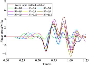
The vertical distance ( $H_{b}$ ) from the model bottom boundary of the model to the tunnel arch is fixed at 6 $B$ . The effect of the side boundary is investigated by changing the horizontal distance ( $W_{b}$ ) from the model side boundary to the tunnel sidewall, which is set to 1 $B$ , 2 $B$ , 3 $B$ , 4 $B$ , 5 $B$ , 6 $B$ , 9 $B$ , 12 $B$ , and 15 $B$ . During the simulation process, the stress time history response of the surrounding rock and soil near the tunnel is analyzed. To ensure the reliability of the results, stress time periods contaminated by reflected waves from the bottom boundary of the model are excluded during data processing. The accuracy of the simulation results is quantitatively assessed by calculated the Pearson correlation coefficient between the stress time history of each case and the corresponding theoretical wave solution. Shear stress results at point B are selected for evaluation (see Fig. 5).

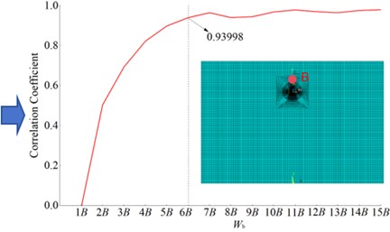
Fig. 5Results of shear stress and correlation coefficients under different model widths: a) time history of shear stress; b) correlation coefficients

Results of shear stress and correlation coefficients under different model widths: a) time history of shear stress; b) correlation coefficients

a)

b)

As shown in Fig. 5, the width of the model has a significant impact on the accuracy of the simulation of the vibration input method in the seismic analysis of tunnels. When the distance $H_{b}$ from the model bottom to the tunnel invert bottom is fixed at 6 $B$ , as the model width increases, the Pearson correlation coefficient between the dynamic responses obtained by the vibration and wave input methods improves in three different stages. That is a rapid improvement stage (a width from 1 $B$ to 2 $B$ , correlation coefficient increases from –0.01093 to 0.50338), a decelerated improvement stage (a width from 2 $B$ to 6 $B$ , correlation coefficient increases from 0.50338 to 0.93998) and a stable convergence stage (width exceeding 6 $B$ , correlation coefficient approaches 1). This behavior is mainly attributed to the attenuation of boundary reflection effects. Therefore, increasing proper model width can effectively improve the simulation accuracy of the vibration input method.

(2) Influence of model height on the calculation accuracy of the vibration input method.

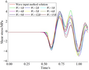
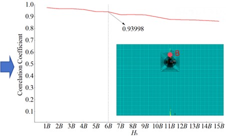
When the lateral boundary distance $W_{b}$ from the model side boundary to the tunnel sidewall is fixed at 6 $B$ , the influence of bottom boundary reflection is examined by changing the vertical distance $H_{b}$ from the model bottom boundary to the tunnel invert bottom (with values of 1 $B$ , 2 $B$ , 3 $B$ , 4 $B$ , 5 $B$ , 6 $B$ , 9 $B$ , 12 $B$ , and 15 $B$ ). To ensure the reliability of the results, signal segments contaminated by bottom boundary reflections are excluded during data processing. The accuracy of the simulation results is quantitatively evaluated by calculating the Pearson correlation coefficient between the simulated stress time history and the corresponding theoretical wave solution. For consistency, representative shear stress results at point B are selected for analysis (see Fig. 6).

As shown in Fig. 6, increasing the model height of a fixed width will result in a slight decrease in the correlation coefficient, although the overall effect is limited. The correlation coefficient between the two methods remains at a high level throughout the entire change process, exceeding 0.8603. The analysis of vibration modes at different heights of the model shows that when the height exceeds a certain threshold, the structure becomes increasingly slender. This leads to a notable change in its natural vibration. These changes, in turn, have a moderate influence on the calculation results.

Fig. 6Results of shear stress and correlation coefficients under different model heights: a) time history of shear stress; b) correlation coefficients

Results of shear stress and correlation coefficients under different model heights: a) time history of shear stress; b) correlation coefficients

a)

b)

(3) Investigation of rational model dimension parameters.

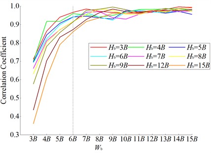
Based on the preceding analysis, a systematic calculation is conducted to evaluate the correlation coefficients between the results of the vibration and wave input methods at different model widths and heights, as shown in Fig. 7. The findings indicate that the height-to-width ratio of the model has a significant impact on the calculation accuracy of the vibration input method. To achieve high simulation accuracy of the vibration input method, especially to maintain a correlation coefficient of above 0.9 relative to the wave input method, a height-to-width ratio of 1:2 is recommended. In addition, the distance from the model side boundary to the tunnel wall, denoted as $W_{b}$ , should be no less than six times the tunnel span. This combination of parameters ensures the calculation efficiency and effectively captures the dynamic interaction behavior between the surrounding rock and the supporting structure.

Fig. 7Correlation coefficients between the vibration and wave input methods under different model widths and model heights

3.3. Analysis of factors influencing the calculation accuracy of the vibration input method under the bedrock surface assumption

The assumption of the bedrock surface is mainly affected by the interference effect caused by the reflected waves generated by the bottom boundary, which affects the calculation accuracy of the vibration input method. According to one-dimensional wave theory, these reflected waves are mainly generated by two key parameters: the propagation speed of seismic waves in rock and soil layers and the model height. Specifically, the velocity of seismic wave directly determines the wave propagation within the medium directly. The model height determines the propagation path and superposition effect of reflected waves. Therefore, to improve the calculation accuracy, it is necessary to conduct a systematic investigation focusing on these two parameters.

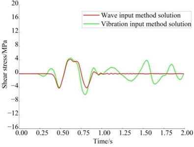
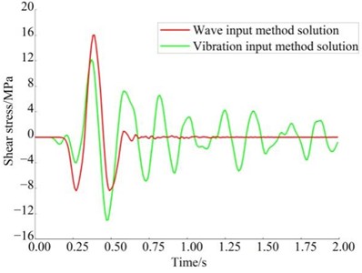
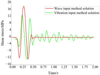
Fig. 8Comparison of shear stress in surrounding rock under different shear wave velocities

a) $c_{s}$ = 200 m/s

b) $c_{s}$ = 400 m/s

c) $c_{s}$ = 600 m/s

The propagation velocity of seismic waves in rock-soil layers is closely related to the surrounding rock. The seismic responses are compared under three wave velocities of 200, 400 and 600 m/s; a model parameter of $W_{b}$ = 8 $B$ , $H_{b}$ = 6 $B$ , and a pulse load duration of 0.25 s. The other geometric parameters are consistent with those in Section 2.3. It is evident that the change in wave velocity have a significant impact on the propagation of seismic waves and the response at observation points (see Fig. 8). The specific results are as follows:

(1) At a wave velocity of 200 m/s, the incident wave passes point completely at 0.915 s, and the reflected wave arrives at 1.455 s, allowing point B to record a complete and undisturbed response segment. This yields a correlation coefficient of 0.89162 with the wave input method;

(2) When the wave velocity increases to 400 m/s, the incident wave passes point B at 0.7075 s, and the reflected wave arrives at 0.7275 s, with a relatively high correlation coefficient of 0.79368 still being maintained between the two methods;

(3) However, at a velocity of 600 m/s, the incident wave passes point B in 0.6383 s. The reflected wave arrives earlier, in 0.485 s, causing significant superposition interference and reducing the correlation coefficient to 0.62837.

This indicates that under high wave velocity in the surrounding rock, the rapid propagation of seismic waves shortens the effective observation time window and increases the difficulty of signal analysis.

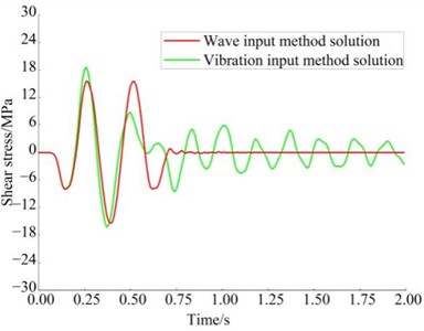
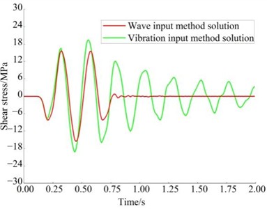
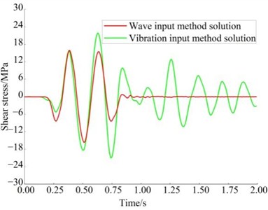
Numerical simulation is used to analyze the seismic response of underlying rock layers at different heights ( $H_{b}$ = 2 $B$ , 4 $B$ , 6 $B$ ) to examine the effect of model height on the reflection behavior at the bedrock interface. The model parameters are set as follows: $W_{b}$ = 8 $B$ and a pulse load duration of 0.5 s. The other geometric parameters are consistent with those in Section 2.3. The rock mass wave velocity is maintained at 400 m/s. The corresponding results are shown in Fig. 9. The findings reveal that when $H_{b}$ = 2 $B$ , the incident wave fully passes point B at 0.5875 s, and the reflected wave arrives at 0.3675 s. The premature arrival of the reflected wave leads to significant superposition interference, resulting in the loss of effective response segments. The correlation coefficient relative to the wave method is only 0.76695. When $H_{b}$ = 4 $B$ , the incident wave completely passes the point at 0.6475 s, and the reflected wave arrives at 0.5475 s. Although the interference in the tail portion of the signal, the number of affected segments decreases and the correlation coefficient increases to 0.86237. When $H_{b}$ = 6 $B$ , the incident wave fully passes the point at 0.7075 s, and the reflected wave arrives at 0.7275 s. Under this condition, a complete interference-free response segment is obtained, and the correlation coefficient reaches 0.91384. These results confirm that increasing the model height can effectively alleviate the reflection effect at the bottom boundary.

Fig. 9Comparison of shear stress in surrounding rock under different model heights

a) $H_{b}$ = 2 $B$

b) $H_{b}$ = 4 $B$

c) $H_{b}$ = 6 $B$

The influence of bedrock surface assumptions on the calculation accuracy of the vibration input method is mainly due to the superposition of incident and reflected waves at the bedrock interface. Since the vibration analysis method usually follows one-dimensional wave theory, the initial time at which reflected waves begin to influence observation points can be estimated based on model height, dynamic loading duration, and wave velocity of the rock and soil medium. Results obtained using the vibration input method before this initial time are accurate and reliable. Therefore, increasing the height of the model appropriately can delay the arrival time of the reflected wave and capture the complete response segment that is not affected by wave superposition, thereby expanding the applicability of the vibration input method.

4. Methodology for delineating and extending the applicability of the vibration input method

4.1. Procedure for delineating and extending applicability

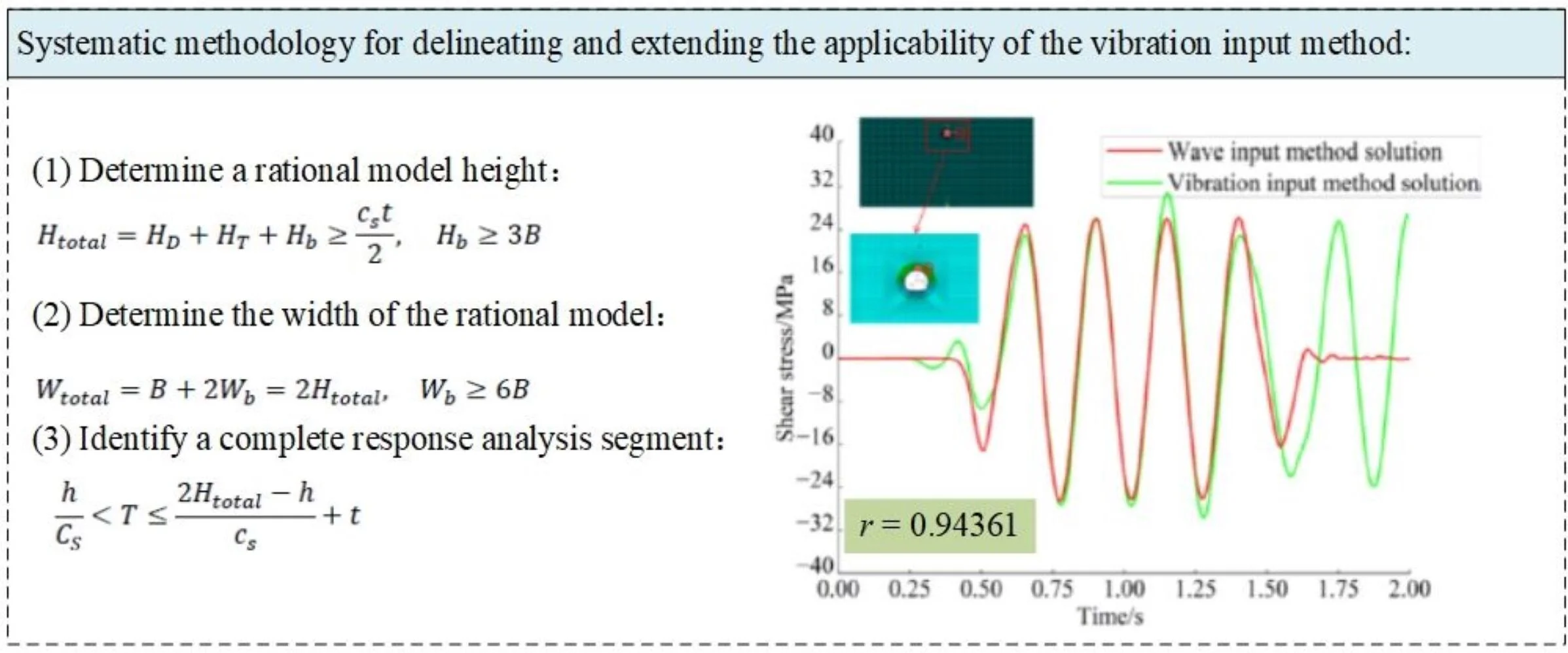
Based on the preceding analysis, the following systematic methodology is proposed for delineating and extending the applicability of the vibration input method:

(1) Determine a rational model height. The height is selected based on the principle of ensuring a complete response segment that is free from interference by reflected waves. The minimum value that satisfies:

10

H_{t o t a l} = H_{D} + H_{T} + H_{b} \geq \frac{c_{s} t}{2}, H_{b} \geq 3 B,

where: $c_{s}$ denotes shear wave velocity, and $t$ represents the duration of the input load.

(2) Determine the width of the rational model based on a prescribed height-to-width ratio of 1:2. The minimum value that satisfies:

11

W_{t o t a l} = B + 2 W_{b} = {2 H}_{t o t a l}, W_{b} \geq 6 B .

(3) Identify a complete response analysis segment. A response analysis segment is identified to ensure that it is complete and free from the influence of reflected waves according to the following criterion:

12

\frac{h}{C_{S}} < T \leq \frac{2 H_{t o t a l} - h}{c_{s}} + t,

where: $T$ is the response analysis time, and $h$ is the height of the study point from the bottom boundary.

4.2. Case study validation

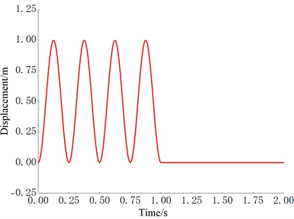
A representative computational case was selected to validate this methodology by simulating a grade VI surrounding rock stratum. The material properties are: elastic modulus $E =$ 0.7168 GPa, Poisson’s ratio $υ =$ 0.4, and density $ρ =$ 1600 kg/m³. Based on elastic theory, the shear wave velocity of the rock stratum is calculated as $v_{s} =$ 400 m/s. The tunnel geometry is defined by a burial depth of $H_{D} =$ 32 m, a span of $B =$ 12 m, and a height of $H_{T} =$ 10 m. The input dynamic load is a pulse wave with a duration of $t =$ 1 s, as shown in Fig. 10.

According to Eq. (10), the total height must satisfy $H_{t o t a l} \geq c_{s} t / 2$ , which equals 200 m. This indicates a minimum overall model height of 200 m, with $H_{b}$ = 160 m ≥ 3 $B$ = 36 m.

From Eq. (11), the minimum overall width of the model is determined to be $W_{t o t a l}$ = 400 m, with $W_{b}$ = (400 − 12)/2 = 194 m, which is greater than 6 $B$ = 72 m.

Based on Eq. (12), the reasonable analysis time interval is derived to be 0.4175 s $< T <$ 1.5825 s.

Fig. 10Dynamic load

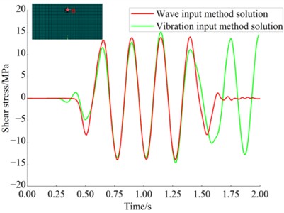
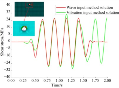
Using this methodology, dimensions are established for the numerical model. Vibration response analysis is conducted for the free-field and scattering field models incorporating tunnel structures. Fig. 11 shows the comparison of the stress response time-history results obtained using the vibration input method and the wave input method.

Fig. 11Comparison of seismic response analysis results for the optimized model: a) free-field model and b) scattered-field model incorporating the tunnel structure

Comparison of seismic response analysis results for the optimized model: a) free-field model and b) scattered-field model incorporating the tunnel structure

a)

b)

Fig. 11 shows the comparative analysis of the stress response time histories at Point B obtained using the vibration input method and the wave input method. As shown in Fig. 5: 1) In the scattered-field model that includes the tunnel lining structure, the shear stress amplitude is more than twice to that of the free-field model. Although the results of the vibration input method slightly increase in amplitude after 1 s, the vibration input method and the wave input method maintain high consistency in the effective analysis time window; 2) The Pearson correlation coefficients are 0.96305 for the free-field model and 0.94361 for the lined tunnel model. These findings confirm that this methodology for defining and extending the applicability of the vibration input method demonstrates satisfactory generalizability and robustness, even for complex models involving a scattered field.

5. Discussion

A comparative analysis was conducted on the vibration input method and wave input method in the tunnel seismic response analysis. Two main mechanisms of errors in the vibration input method were determined: the coupling effect between the lateral boundary of the model and the natural vibration characteristics of the structure, as well as the standing wave effect caused by the fully fixed basal boundary conditions. Combined the optimization of model size with the identification of effective analysis time windows, a strategy for extending the applicability of the vibration input method was proposed. Although the results provide a quantitative basis for the rational application of the vibration input method in tunnel seismic analysis, there are several key aspects worth further discussion.

To isolate the main error mechanisms, a linear elastic constitutive model is adopted to eliminate the interference of material damping on wave-field attenuation and accurately identified boundary reflections and standing wave effects. Although this assumption is reasonable for mechanism-oriented investigations, caution must be exercised when extrapolating quantitative conclusions (such as the recommended optimal height-to-width ratio) to practical engineering contexts. In this regard, it is fully acknowledged that the nonlinear behavior of actual surrounding rock introduces damping effects that attenuate reflected wave amplitudes. It may objectively extend the applicable analysis time of the vibration input method, although the mitigation of the lateral boundary coupling effect is limited. Based on the mechanical framework, systematic sensitivity analysis on various constitutive models will be conducted to quantify the correction coefficients of applicability standard formulas.

It should also be noted that this study used single frequency pulse excitation to elucidate the potential mechanism. This simplification has been proven effective in deriving the conceptual standard formulas (Eqs. (10-12)). However, for real ground motions such as the El Centro record, their broad spectral composition may excite multi-modal resonance with the model, thereby changing the timing of peak responses and affecting the selection of optimal time windows. Therefore, future parameter sensitivity analysis based on standard seismic records will be conducted to improve the engineering applicability of this method.

For deep buried long tunnels or prolonged strong earthquake events, the model size calculated by this formula may become too large, resulting in high calculation. To solve this, a hybrid strategy combining vibration input method with viscous spring base boundary and coordinate transformation can be explored. This strategy is expected to completely eliminate standing wave pollution. However, this requires are-establishment of the theoretical framework for the application of equivalent nodal forces, which is a key direction of our future research.

6. Conclusions

This study systematically evaluated the accuracy of the vibration input method and its influencing factors in seismic response analysis of tunnels to assess its applicability and the development of model optimization strategies. The main conclusions are as follows:

1) The simulation accuracy of the vibration input method in tunnel seismic analysis is generally lower than that of the wave input method. This difference is mainly due to two sources of error: the coupling effect between the model side boundary and the inherent vibration characteristics of the structure, and the standing wave effect caused by the reflection of the bottom boundary.

2) Based on the results of the wave input method, the correlation between the two methods shows a clear trend as the geometric shape of the model changes. When the height of the model is fixed, as the width of the model increases, the correlation coefficient shows three stages of change: “rapid increase-deceleration growth-asymptotic convergence to 1”. When the width of the model is fixed, the correlation coefficient shows a trend of “approximately stable slightly decreasing” with increasing height. Based on parameter sensitivity analysis, the reasonable aspect ratio for the vibration input method model is determined to be 1:2. In addition, the distance W-b from the model boundary to the tunnel sidewall should not be less than six times the tunnel span.

3) Assuming that the influence of bedrock surface on the accuracy of vibration input method calculation mainly comes from the superposition of reflected bedrock waves and incident waves. The superposition interval begins when the reflected wave arrives at the observation point and ends when the incident wave passes it. These critical times can be approximated using one-dimensional wave theory. The superposition interval starts from the arrival of the reflected wave at the observation point and ends when the incident wave passes through the observation point. These critical times can be approximated using one-dimensional wave theory. To obtain a complete response segment unaffected by this superposition, the application of the vibration input method can be extended by increasing the model height, which delays the arrival time of the reflected wave. To obtain a complete response segment that is not affected by this superposition, the applicability of the vibration input method can be expanded by increasing the model height, which will delay the arrival time of the reflected wave.

4) A methodology for defining and extending the scope of the vibration input method is proposed. It includes a three-step process: first, establish sufficient model height to ensure that the complete response segment is not affected by reflected waves; second, determine the appropriate model width based on a recommended aspect ratio of 1:2; and third, identify a complete and effective response analysis section that is not affected by reflected wave interference.

References

G. Tsinidis et al., “Seismic behaviour of tunnels: from experiments to analysis,” Tunnelling and Underground Space Technology, Vol. 99, p. 103334, Feb. 2020, https://doi.org/10.1016/j.tust.2020.103334

Publisher
L. Guo, Y. Shen, M. Lyu, D. Zhang, and Z. Huang, “Non-parametric seismic fragility assessment of underground structures incorporating stochastic ground motion,” Soil Dynamics and Earthquake Engineering, Vol. 200, No. Part B, p. 109893, Nov. 2025, https://doi.org/10.1016/j.soildyn.2025.109893

Publisher
E. Sandoval and A. Bobet, “Effect of input frequency on the seismic response of deep circular tunnels,” Soil Dynamics and Earthquake Engineering, Vol. 139, p. 106421, Sep. 2020, https://doi.org/10.1016/j.soildyn.2020.106421

Publisher
M. Eskandarighadi, C. R. Mcgann, and C. A. de La Torre, “2D site response modeling of the Treasure Island vertical array considering spatially varying input motions with non-vertical incidence,” Soil Dynamics and Earthquake Engineering, Vol. 200, No. Part B, p. 109878, Oct. 2025, https://doi.org/10.1016/j.soildyn.2025.109878

Publisher
H. Mashhadban, A. J. Choobbasti, I. Shooshpasha, and M. Ashtiani, “Evaluation of the seismic response of the slopes in the presence of the horseshoe tunnel,” Bulletin of Engineering Geology and the Environment, Vol. 80, No. 1, pp. 157–177, Jul. 2020, https://doi.org/10.1007/s10064-020-01920-w

Publisher
C. Shi, L. Tao, P. Ding, Z. Wang, Z. Jia, and M. Shi, “Analytical solution for deep non-circular tunnels considering slippage effects under far-field seismic SV waves,” Tunnelling and Underground Space Technology, Vol. 144, p. 105552, Dec. 2023, https://doi.org/10.1016/j.tust.2023.105552

Publisher
M. Yadav, A. Tyagi, and V. A. Sawant, “Seismic response of shallow circular tunnel in stratified soil with interbedded liquefiable sandy and silty soils,” Tunnelling and Underground Space Technology, Vol. 166, p. 106954, Aug. 2025, https://doi.org/10.1016/j.tust.2025.106954

Publisher
W. B. Jing, Z. Wang, L. P. Jing, and W. H. Qi, “Seismic motion input methods of viscous-elastic boundary and numerical simulation of seismic response on large diameter tunnels,” (in Chinese), Progress in Earthquake Sciences, Vol. 55, No. 3, pp. 125–134, 2025, https://doi.org/10.19987/j.dzkxjz.2024-013

Publisher
S. Kontoe, L. Zdravkovic, and D. M. Potts, “An assessment of the domain reduction method as an advanced boundary condition and some pitfalls in the use of conventional absorbing boundaries,” International Journal for Numerical and Analytical Methods in Geomechanics, Vol. 33, No. 3, pp. 309–330, Feb. 2009, https://doi.org/10.1002/nag.713

Publisher
H. T. Yu, Y. S. Yang, Y. Yuan, K. P. Duan, and Q. Gu, “A comparison between vibration and wave methods in seismic analysis of underground structures,” (in Chinese), China Earthquake Engineering Journal, Vol. 41, No. 4, p. 845, 2019, https://doi.org/10.3969/j.issn.1000-0844.2019.04.845

Publisher
J. M. Mayoral and G. Mosqueda, “Seismic interaction of tunnel-building systems on soft clay,” Soil Dynamics and Earthquake Engineering, Vol. 139, p. 106419, Sep. 2020, https://doi.org/10.1016/j.soildyn.2020.106419

Publisher
S. Kömürcü, Balık, and B. Işık, “Examination of the earthquake-induced failure mechanism of intentionally damaged rammed earth walls via shaking table experiments,” Engineering Failure Analysis, Vol. 185, p. 110397, Nov. 2025, https://doi.org/10.1016/j.engfailanal.2025.110397

Publisher
Z. D. Ding, Y. S. Chen, and H. Zi, “Study on artificial boundaries and ground motion input method in tunnel seismic response,” (in Chinese), Earthquake Engineering and Engineering Dynamics, Vol. 42, No. 3, pp. 52–61, 2022, https://doi.org/10.13197/j.eeed.2022.0306

Publisher
J. H. Wang, X. J. Zhou, L. L. Mao, and H. Y. Hu, “Comparative study of earthquake input methods for the seismic analysis of underground structures,” (in Chinese), Modern Tunnelling Technology, Vol. 52, No. 3, pp. 103–109, 2015, https://doi.org/10.13807/j.cnki.mtt.2015.03.015

Publisher
H. Jiao, M. Zhao, J. Huang, X. Zhao, and X. Du, “Nonlinear response of tunnel portal under earthquake waves with different vibration directions,” Computer Modeling in Engineering and Sciences, Vol. 131, No. 3, pp. 1289–1314, 2022, https://doi.org/10.32604/cmes.2022.018540

Publisher
Y. S. Yang, H. T. Yu, and Y. Yuan, “A seismic analysis model of underground structure with elastic base condition,” (in Chinese), Chinese Journal of Underground Space and Engineering, Vol. 16, No. 4, pp. 1096–1101, 2020, https://doi.org/10.20174/j.juse.2020.04.017

Publisher
R. L. Kuhlemeyer and J. Lysmer, “Finite element method accuracy for wave propagation problems,” Journal of the Soil Mechanics and Foundations Division, Vol. 99, No. 5, pp. 421–427, 2021, https://doi.org/10.1061/jsfeaq.0001885

Publisher

About this article

Received

December 29, 2025

Accepted

July 28, 2026

Published

August 19, 2026

SUBJECTS

Seismic engineering and applications

DOI

https://doi.org/10.21595/jve.2026.25948

Keywords

seismic response of tunnels

vibration input method

assessment of accuracy

applicability boundaries

optimized numerical model

Acknowledgements

This work was supported by the Natural Science Foundation of Chongqing (Grant No. CSTB2023NSCQ-MSX0503), the Science and Technology Research Program of Chongqing Municipal Education Commission (Grant No. KJQN202500728), and the Science and Technology Research Project of Chongqing Education Commission (Grant No. KJZD-M202400702).

Data Availability

The datasets generated during and/or analyzed during the current study are available from the corresponding author on reasonable request.

Author Contributions

Xukai Tan: conceptualization, methodology, software, formal analysis, writing-original draft, funding acquisition, resources. Jiamu Yuan: investigation, formal analysis, writing-review and editing. Guangping Lu: investigation, project administration. Feng Gao: resources, methodology, writing-review and editing. Hao Ding: resources, methodology, writing-review and editing. Zhengdong Chen: investigation, writing-review and editing.

Conflict of interest

The authors declare that they have no conflict of interest.

This is an open access article distributed under the Creative Commons Attribution License (CC BY 4.0), which permits unrestricted use, distribution, and reproduction in any medium, provided the original work is properly cited.

X. Tan, Z. Chen, J. Yuan, G. Lu, F. Gao, and H. Ding, “Error mechanisms and applicability boundaries of the vibration input method in tunnel seismic response analysis,” Journal of Vibroengineering, Vol. 28, No. 7, –16, Aug. 2026, https://doi.org/10.21595/jve.2026.25948

Copy Extrica

Copied to clipboard!

TY  - JOUR
DO  - 10.21595/jve.2026.25948
UR  - https://doi.org/10.21595/jve.2026.25948
TI  - Error mechanisms and applicability boundaries of the vibration input method in tunnel seismic response analysis
T2  - Journal of Vibroengineering
AU  - Tan, Xukai
AU  - Chen, Zhengdong
AU  - Yuan, Jiamu
AU  - Lu, Guangping
AU  - Gao, Feng
AU  - Ding, Hao
PY  - 2026
DA  - 2026/08/19
PB  - Extrica
VL  - 28
IS  - 7
SN  - 1392-8716
SN  - 2538-8460
ER  - 

Copy Ris

Copied to clipboard!

@article{doi_10.21595/jve.2026.25948,
  title = {Error mechanisms and applicability boundaries of the vibration input method in tunnel seismic response analysis},
  author = {Tan, Xukai and Chen, Zhengdong and Yuan, Jiamu and Lu, Guangping and Gao, Feng and Ding, Hao},
  journal = {Journal of Vibroengineering},
  year = {2026},
  month = {8},
  volume = {28},
  number = {7},
  doi = {10.21595/jve.2026.25948},
  url = {https://doi.org/10.21595/jve.2026.25948},
  publisher = {Extrica},
  issn = {1392-8716},
  eissn = {2538-8460},
}

Copy Bibtex

Copied to clipboard!

[1]X. Tan, Z. Chen, J. Yuan, G. Lu, F. Gao, and H. Ding, “Error mechanisms and applicability boundaries of the vibration input method in tunnel seismic response analysis,” Journal of Vibroengineering, Aug. 2026, doi: 10.21595/jve.2026.25948.

Copy IEEE

Copied to clipboard!

Tan, Xukai, Zhengdong Chen, Jiamu Yuan, Guangping Lu, Feng Gao, and Hao Ding. “Error mechanisms and applicability boundaries of the vibration input method in tunnel seismic response analysis.” Journal of Vibroengineering 28, no. 7 (2026). https://doi.org/10.21595/jve.2026.25948.

Copy Chicago

Copied to clipboard!

Error mechanisms and applicability boundaries of the vibration input method in tunnel seismic response analysis

Abstract

Highlights

1. Introduction

2. Implementation methods and a comparative analysis of wave input method and vibration input method

2.1. Implementation of the wave input method

2.2. Implementation of the vibration input method

2.3. Comparative analysis of vibration and wave input methods

3. Sensitivity analysis of the accuracy of the vibration input method with respect to various influencing factors

3.1. Pearson correlation coefficient

3.2. Investigation of the influence of model dimensions on the accuracy of the vibration input method

3.2.1. Calculation cases

3.2.2. Analysis of calculation results

3.3. Analysis of factors influencing the calculation accuracy of the vibration input method under the bedrock surface assumption

4. Methodology for delineating and extending the applicability of the vibration input method

4.1. Procedure for delineating and extending applicability

4.2. Case study validation

5. Discussion

6. Conclusions

References

About this article

Related Articles