Uncertain RUL prediction for aircraft engines: an attention-based ensemble method with partial-transfer Bayesian deep learning

Zeng, Jiyan; Tong, Yaohua; Cheng, Yujie; Lu, Chen

doi:10.21595/jve.2026.26015

Journal of Vibroengineering

Browse Journal

Submit article

Published: April 21, 2026

Check for updates

Uncertain RUL prediction for aircraft engines: an attention-based ensemble method with partial-transfer Bayesian deep learning

Jiyan Zeng¹

Yaohua Tong²

Yujie Cheng³

Chen Lu⁴

^{1, 3, 4}The School of Reliability and Systems Engineering, Beihang University, Beijing, China

^{1, 3, 4}The Science and Technology Laboratory on Reliability and Environmental Engineering, Beihang University, Beijing, China

²National Superior College for Engineers, Beihang University, Beijing, China

^{3, 4}Hangzhou International Innovation Institute, Beihang University, Hangzhou, China

Corresponding Author:

Yujie Cheng

Cite the article Download PDF

Article in Press

Downloads 0

Abstract

Accurate prediction of the remaining useful life (RUL) of aircraft engines is crucial for ensuring flight safety and optimizing maintenance strategies. However, traditional data-driven methods typically yield point estimation, failing to quantify uncertainties arising from data noise and model limitations. This study proposes an attention-based ensemble method with partial-transfer Bayesian deep learning (Att-ensembled PT-BDL) for uncertainty quantification in aircraft engine RUL prediction. The proposed method transfers weights and biases from existing point estimation deep learning models as prior knowledge to the mean values of weights and biases in Bayesian deep learning models, freezing these parameters during training to reduce trainable parameters and enhance computational efficiency. An ensemble framework, enhanced by an attention mechanism, integrates multiple models to improve prediction accuracy and uncertainty quantification performance. A case study is conducted to demonstrate the effectiveness of the proposed method with a dataset of the PHM data challenge. The experiment results show that the proposed Att-ensembled PT-BDL method can achieve a better prediction accuracy and uncertainty quantification performance in terms of root mean square error (RMSE), prediction interval coverage probability (PICP) and prediction interval normalized average width (PINAW).

1. Introduction

Remaining useful life (RUL) prediction of aircraft engines is critical for ensuring flight safety and optimizing maintenance decisions [1]. Accurate RUL prediction can effectively mitigate the risk of unexpected failures, extend equipment lifespan, and reduce operational costs for airlines [2]. Traditional RUL prediction methods can be categorized into knowledge-based methods, model-driven methods and data-driven methods [3]. Among these methods, data-driven methods have become predominant in aircraft engine RUL prediction due to advancements in sensor technology, data acquisition and data processing, enabling effective feature extraction from complex, high-dimensional data [4].

However, most existing data-driven RUL prediction methods provide results in the form of point estimation [5], [7]. Due to noise in data acquisition, the complexity of operating conditions, and inherent limitations of predictive models, these point estimations are often accompanied by uncertainty [8]. Such uncertainty can lead to suboptimal maintenance decisions, thereby increasing costs and even leads to safety risks. Consequently, quantifying uncertainty in RUL predictions has emerged as a critical research focus in the field of prognostics and health management to support more reliable maintenance strategies.

Exploiting the posterior probability computation capability of Bayesian methods, researchers have proposed Bayesian machine learning to incorporate probabilistic distributions for characterizing model parameter uncertainty [9]. To address this, researchers have proposed Bayesian machine learning methods, which incorporate probabilistic distributions to characterize model parameter uncertainty [10]. Further advancements have led to Bayesian Deep Learning (BDL), which extends traditional deep learning by replacing neurons with parameters for weights and biases, with Bayesian neurons parameterized by weight means, weight variances, bias means, and bias variances, enabling uncertainty quantification in RUL predictions [11]. However, BDL methods introduce additional trainable parameters (weight and bias variances), significantly increasing computational complexity and training challenges, particularly when training data is limited, which often results in suboptimal performance [12].

In practical industrial applications, aircraft engines often have pre-existing RUL point estimation models based on traditional deep learning, which encapsulate valuable prior knowledge [13]. However, most BDL methods build models from scratch, failing to leverage this prior knowledge, leading to inefficient training and resource waste, particularly when training data is limited.

Besides, a single BDL model may lack universality for the complex operation condition of aircrafts, which further decreases prediction and uncertainty quantification performance. In face of this problem, researchers have introduced ensemble learning into RUL prediction [14]. Li et al. [14] modeled an exponential wear degradation process using an ensemble learning-based prognostic method and predicted the RUL of aircraft engines. Ordóñez et al. [15] uses the output of autoregressive integrated moving average (ARIMA) as the input of support vector machine (SVM) to predict the RUL of aircraft engines. Ensemble learning methods have been proved can fuse the advantages of its member algorithms and achieve better performance.

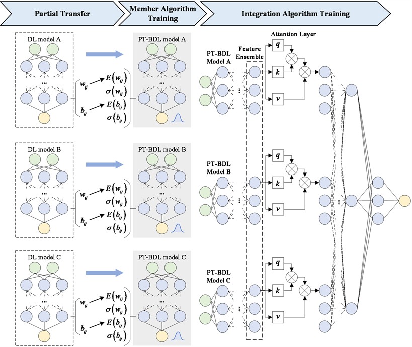
To address these challenges, this study proposes an attention-based ensemble method with partial-transfer Bayesian deep learning (Att-ensembled PT-BDL) for uncertainty quantification in aircraft engine RUL prediction. The Att-ensembled PT-BDL framework comprises three key steps: partial transfer, member algorithm training, and integration algorithm training. In the partial transfer step, weights and biases from pre-existing deterministic deep learning models are transferred as prior knowledge to initialize the mean values in Bayesian deep learning (BDL) models with identical structures. These mean parameters are frozen during training, while only the variances are optimized, halving the trainable parameters and enhancing computational efficiency. In the member algorithm training step, three diverse partial-transfer BDL models serve as base learners: (1) PT-LSTM, built on LSTM with Bayesian gates (forget, input, output) to capture temporal dependencies; (2) PT-CNN, employing Bayesian convolutional and linear layers for multi-dimensional feature extraction; (3) PT-SAE, a symmetric auto-encoder with Bayesian encoder-decoder for high-level feature compression. Training minimizes a loss combining mean squared error (MSE) and Kullback-Leibler (KL) divergence, with gradients backpropagated solely to variances. In the integration algorithm training step, features from the last hidden layers of the PT-BDL models are concatenated and fed into an attention layer with trainable query, key, and value parameters for feature weighting and optimization. This is followed by a Bayesian regressor to produce uncertain RUL predictions. The approach seamlessly extends to federated learning by partially transferring from collaboratively trained point-estimate models, enabling privacy-preserving uncertainty quantification without raw data sharing.

The main contributions of this paper are the following:

– A partial-transfer Bayesian deep learning (PT-BDL) mechanism that initializes the expected weights and biases of Bayesian neurons using parameters from pre-trained deterministic deep learning models while freezing these mean parameters during training and only optimizing variances, which can lower computational cost and enable efficient uncertainty modeling with insufficient data.

– An attention-based ensemble integration framework that fuses feature representations extracted from the last hidden layers of multiple heterogeneous PT-BDL models (PT-LSTM, PT-CNN, and PT-SAE). A trainable attention layer dynamically evaluates and reweights these features using learned query, key, and value parameters, followed by a Bayesian regressor to produce calibrated uncertain RUL predictions.

– A complete training paradigm combining MSE loss with KL divergence for member PT-BDL models and a multi-metric evaluation (RMSE, PICP, PINAW) for the integrated output, ensuring both predictive accuracy and reliable uncertainty quantification in aircraft engine RUL prognosis.

The remainder of this paper is organized as follows. Related work of this study is introduced in Section 2. The proposed attention-based ensemble method with partial-transfer Bayesian deep learning is detailed in Section 3. A case study conducted to quantify uncertainty in C-MAPSS dataset using the proposed method is presented in Section 4. The conclusions of this study are provided in Section 5.

2. Related work

2.1. Bayesian deep learning for uncertainty quantification

Bayesian [20] inference is grounded in conditional probability, which quantifies the probability of an event A given evidence B as:

1

P (A| B) = \frac{P (A B)}{P (B)},

where $P (A, B)$ is the joint probability. This forms the basis of Bayes' theorem, central to updating beliefs with data:

2

P (A| B) = \frac{P (B| A) P (A)}{P (B)},

where $P (A | B)$ is the posterior over parameters $A$ , $P (B | A)$ is the likelihood, $P (A)$ is the prior, and $P (B)$ is the evidence (marginal likelihood). In deep learning, this extends to probabilistic modeling of neural networks, leading to Bayesian deep learning (BDL) [21].

In BDL, the predictive distribution for a new input $x^{*}$ incorporates uncertainty by marginalizing over the posterior:

3

p (y^{*}| x^{*}, B) = \int p (y^{*}| x^{*}, A) p (A| B) d A .

Since the posterior is intractable, variational inference approximates it with $q_{ϕ} (A)$ , maximizing the evidence lower bound (ELBO):

4

L_{E L B O} = E_{q_{ϕ} (A)} [\log p (B | A)] - K L (q_{ϕ} (A) | | p (A)) .

This yields both aleatoric (data noise) and epistemic (model uncertainty) components, enabling calibrated prediction intervals for RUL. Monte Carlo dropout offers a practical approximation by randomly masking weights during inference to sample from the posterior, facilitating uncertainty estimation without full Bayesian computation.

In PHM, BDL has been extensively applied to generate probabilistic RUL forecasts. For instance, Bayesian neural networks with Monte Carlo dropout have been used for RUL prediction in aircraft engines, incorporating uncertainty for unlabeled run-to-failure data. A hybrid Bayesian deep learning model combines LSTM autoencoders with Bayesian layers for enhanced prognostics, achieving better calibration on turbofan datasets. Frameworks like Bayesian convolutional LSTMs decompose predictive variance, while adversarial Transformers address long-term uncertainty in RUL tasks. Benchmarks emphasize BDL's role in decision-making under uncertainty, but highlight challenges in hyperparameter tuning for aviation systems. However, each weight connection requires four parameters ( $μ_{w}, σ_{w}^{2}, μ_{b}, σ_{b}^{2}$ ), doubling the parameter count and computational cost compared to deterministic models. This overhead severely limits scalability in real-time aviation monitoring with constrained data, often leading to overfitting or prolonged training times.

2.2. Transfer learning in RUL prediction

Transfer learning leverages pre-trained models to initialize target tasks, mitigating data scarcity and domain shift [22]. In its foundational form, it involves knowledge transfer from a source domain with abundant labeled data to a target domain with limited or unlabeled samples [23]. This is particularly useful in RUL prediction, where collecting comprehensive run-to-failure data for aircraft engines is expensive and time-consuming due to long operational cycles and safety constraints. Given a source model with parameters $θ_{s}$ trained on a related domain, fine-tuning adapts a subset of layers to the target task:

5

\min_{θ_{t}} L (θ_{t} {; D}_{t}), s . t . θ_{s}^{(l)} = θ_{s}^{(l)} \forall l \leq L_{f},

where $θ_{t}$ denotes the parameters of the target model, $L ({; D}_{t})$ is the loss function evaluated on the target dataset $D_{t}$ , $l$ represents the layer index, and $L_{f}$ is the frozen layer index (i.e., layers $l \leq L_{f}$ are kept fixed to preserve general features learned from the source domain, while higher layers are updated to adapt to the target task).

Domain adaptation further aligns feature distributions to handle discrepancies between source and target data distributions, often using discrepancy metrics like maximum mean discrepancy (MMD):

6

M M D^{2} (Χ_{s}, Χ_{t}) = {‖\frac{1}{n_{s}} \sum_{i = 1}^{n_{s}} ϕ (x_{s}^{i}) - \frac{1}{n_{t}} \sum_{j = 1}^{n_{t}} ϕ (x_{t}^{j})‖}_{H}^{2},

where, $X_{s}$ and $X_{t}$ are the source and target feature sets, $n_{s}$ and $n_{t}$ are the number of samples in each domain, $x_{s}^{i}$ and $x_{t}^{j}$ are individual feature vectors, $ϕ$ maps features to a reproducing kernel Hilbert space $Η$ , allowing non-linear alignment. Adversarial techniques, such as domain-adversarial neural networks (DANN), minimize domain shift by incorporating a gradient reversal layer to fool a domain discriminator, effectively learning domain-invariant features during joint training of the feature extractor and task classifier.

Transfer learning is widely used in RUL prediction to reduce training data requirements by 70-90 % via fine-tuning and domain alignment. However, applications to BDL remain limited; variational parameters are typically reinitialized from scratch, failing to exploit priors from pre-existing deterministic RUL models, resulting in inefficient training.

2.3. Attention-based ensemble learning in RUL prediction

Ensemble learning enhances robustness by aggregating predictions from diverse base learners. The foundational principle is to combine multiple weak models to form a strong predictor, reducing overall variance and bias through averaging or voting mechanisms. Deep ensembles provide uncertainty estimates via Monte Carlo sampling across independently trained networks, capturing model diversity:

7

{\hat{y}}_{e n s} = \frac{1}{M} \sum_{m = 1}^{M} f_{θ_{m}} (x),

8

σ_{e n s}^{2} = \frac{1}{M} \sum_{m = 1}^{M} (f_{θ_{m}} (x) - {\hat{y}}_{e n s})^{2},

where $M$ is the number of ensemble members, $f_{θ_{m}}$ is the $m$ -th base model with parameters $θ_{m}$ , $x$ is the input, ${\hat{y}}_{e n s}$ is the ensemble mean prediction, and $σ_{e n s}^{2}$ is the predictive variance reflecting model disagreement.

Attention mechanisms improve feature-level fusion by computing dynamic weights, allowing the model to focus on relevant parts of the input [24]. Inspired by human attention, it assigns higher weights to important features while suppressing noise [25]. For feature-level ensemble of $K$ base models with hidden representations $h_{k}$ , the attention score for model $k$ is computed using scaled dot-product attention:

9

α_{k} = \frac{\exp (q^{T} K_{k} / \sqrt{d})}{\sum_{j = 1}^{K} \exp (q^{T} K_{j} / \sqrt{d})},

10

h_{f u s e d} = \sum_{k = 1}^{K} α_{k} V_{k},

where $K$ is the number of base models, $h_{k}$ is the hidden representation from the $k$ -th model, $q$ is the query vector, $K_{k}$ and $V_{k}$ are the key and value projections of $h_{k}$ , $d$ is the dimension of the key vectors (scaling by $\sqrt{d}$ prevents vanishing gradients in softmax), $α_{k}$ is the attention weight, and $h_{f u s e d}$ is the fused feature.

Multi-objective optimization can further balance ensemble diversity to encourage disagreement among bases and minimize loss on validation data to improve accuracy.

Attention-based ensembles are effective for deterministic RUL prediction by focusing on degradation-critical features and reducing model bias. However, they do not propagate uncertainty through attention weights or ensemble variance, and integration with partial-transfer Bayesian models remains unexplored.

3. Methodology

In this study, an attention-based ensemble method with partial-transfer Bayesian deep learning (Att-ensembled PT-BDL) is proposed for uncertain RUL prediction. The Att-ensembled PT-BDL method contains three steps, which are partial transfer, member algorithm training and integration algorithm training. The framework of the proposed method is shown in Fig. 1.

In the partial transfer step, the prior knowledge of well-trained deep-learning (DL) models is partially transferred to PT-BDL models. Specifically, PT-BDL models are of the same structure as the DL models. Weights $w$ and biases $b$ of all neurons in DL models are used as initial values of expected weights $E (w)$ and biases $E (b)$ of corresponding neurons in PT-BDL models, while variance of weights $σ (w)$ and biases $σ (b)$ in PT-BDL models are randomly initialized.

In the member algorithm training step, expected weights $E (w)$ and biases $E (b)$ in PT-BDL models are frozen to their initial values while variances of weights $σ (w)$ and biases $σ (w)$ are trained normally. There are two reasons why freeze-tuning instead of full-tuning is chosen. The first reason is that scenario of the source model is highly similar to the scenario of the target model while the other reason is that training data of the target model is insufficient.

In the training process, the loss function is calculated in terms of both mean square error (MSE) and KL divergence. During the back propagation, gradients of expected weights $E (w)$ and biases $E (b)$ are set to 0 while gradients of variances of weights $σ (w)$ and biases $σ (b)$ are loss times partial derivative $\frac{\partial E}{\partial σ}$ .

In the integration algorithm training step, features extracted with PT-BDL models, which are output of the last hidden layers of PT-BDL models, are used as the input of the attention-based integration algorithm. The first layer of the attention-based integration algorithm is an attention layer, where three trainable parameters $q$ , $k$ and $v$ are trained for feature evaluation and optimization. The attention layer is followed by a Bayesian regressor, which maps optimized features to the corresponding uncertain RUL.

Fig. 1The framework of the Att-ensembled PT-BDL method

3.1. Partial transfer

In the partial transfer step, existing DL models are used to construct Bayesian deep learning models with partial transfer learning. The constructed PT-BDL models are of the same structure as their corresponding DL models, including the same input dimension, output dimension, number of hidden layers, type of hidden layers and number of neurons in each layer. The prior knowledge of existing DL models (source models), which are weights $w$ and biases $b$ of all neurons, are transferred to PT-BDL models (target models) as expected weights $E (w)$ and biases $E (b)$ . Different from traditional transfer learning, only a part of trainable parameters in target PT-BDL models are transferred to, while the other part of trainable parameters (variances of weights $σ (w)$ and biases $σ (b)$ ) are normally initialized and trained. The PT-BDL models contains only half number of trainable parameters compared with Bayesian deep learning models of the same structure, which means the PT-BDL models can largely reduce the computing resource consumption. However, due to the non-linearity of deep learning models, PT-BDL models may give biased prediction results even if results of the corresponding DL models are unbiased.

To reduce the influence of biased prediction results, the ensemble learning framework is introduced into the proposed method. Three PT-BDL models of the different type are constructed as member algorithms, which are partial transfer Bayesian long short-term memory model (PT-LSTM), partial transfer Bayesian convolutional neural network model (PT-CNN) and partial transfer Bayesian stacked auto-encoder model (PT-SAE).

3.1.1. The PT-LSTM model

The PT-LSTM model is constructed based on traditional LSTM model. Like the LSTM model, the PT-LSTM is structured by several units, each of which contains three gates, which are Bayesian forget gate, Bayesian input gate, and Bayesian output gate [26].

At the forget gate, $f_{t}$ can be obtained in the following way:

11

f_{t} = s i g m o i d (w_{f} ∙ x_{t} + u_{f} ∙ h_{t - 1} + b_{f}),

where $x_{t}$ is the data at time $t$ , $h_{t - 1}$ is the output at time $t - 1$ , $w_{f}$ and $u_{f}$ are sampled from gaussian distributions $μ (E (w_{f}), σ (w_{f}))$ and $μ (E (u_{f}), σ (u_{f}))$ , $b_{f}$ is sampled from $μ (E (b_{f}), σ (b_{f}))$ .

At the input gate, $i_{t}$ and ${\tilde{C}}_{t}$ can be obtained in the following way:

12

i_{t} = s i g m o i d (w_{i} ∙ x_{t} + u_{i} ∙ h_{t - 1} + b_{i}),

13

{\tilde{C}}_{t} = \tanh (w_{c} ∙ x_{t} + u_{c} ∙ h_{t - 1} + b_{c}),

where $w_{i}$ , $u_{i}$ , $b_{i}$ , $w_{c}$ , $u_{c}$ and $b_{c}$ are sampled from corresponding distributions.

At the output gate, by integrating $f_{t}$ , $i_{t}$ , ${\tilde{C}}_{t}$ and the state value $C_{t - 1}$ of the unit at time $t - 1$ , the unit’s state value $C_{t}$ at time $t$ can be obtained as follows:

14

C_{t} = f_{t} \times C_{t - 1} + i_{t} \times {\tilde{C}}_{t} .

Combining $C_{t}$ , $x_{t}$ and $h_{t - 1}$ , output at time $t$ can be obtained:

15

O_{t} = s i g m o i d (w_{0} ∙ x_{t} + u_{0} ∙ h_{t - 1} + b_{0}),

16

h_{t} = O_{t} ∙ t a n h (C_{t}),

where $w_{0}$ , $u_{0}$ and $b_{0}$ are sampled from corresponding distributions.

3.1.2. The PT-CNN model

The PT-CNN model is constructed based on traditional CNN model. The traditional CNN model contains convolutional layers, which uses convolution operation instead of general matrix multiplication. This makes CNN model suitable for extracting features from multiple array data [27].

Similar with traditional CNN models, the PT-CNN model contains Bayesian convolutional layers (BCNN), pooling layers and Bayesian linear layers (Blinear), in which BCNN layers and pooling layers are core components.

In BCNN layers, the output is calculated with convolution operations:

17

y_{i} = σ (\sum_{r = 1}^{F} w_{r} ∙ x_{(r + i \times S)} + b) F,

18

0 \leq i \leq \frac{H d}{S},

where $y_{i}$ is the output of a node in the BCNN layer, $w_{r}$ and $b$ are sampled from corresponding distributions, $F$ , $S$ and $H d$ are the kernel size, the stride length and the length of the input data separately.

The PT-CNN model uses convolution to fuse feature from high dimensional data, granting it the ability to quantify uncertainty in aircraft engine RUL.

3.1.3. The PT-SAE model

The PT-SAE model a symmetric Bayesian neural network consists of Bayesian encoders and Bayesian decoders. The Bayesian encoder compresses input data to extract features, and the Bayesian decoder reconstructs the input data from the extracted feature, which ensures the Bayesian encoder can extract features from the input data with minimum information loss.

In the Bayesian encoder:

19

z = σ_{1} (w_{1} ∙ x + b_{1}),

where $x$ is the input data, $z$ is the extracted feature, $w_{1}$ and $b_{1}$ are sampled from corresponding distributions and $σ_{1}$ is the activation function of encoder.

In the Bayesian decoder:

20

y = σ_{2} (w_{2} ∙ z + b_{2}),

where $y$ is the reconstructed data, $w_{2}$ and $b_{2}$ are sampled from corresponding distributions and $σ_{2}$ is the activation function of decoder.

The PT-SAE model can extract high-level features better, making it suitable for aircraft engine RUL uncertainty quantification.

3.2. Member algorithm training

In the member algorithm training step, the member algorithms constructed in the previous step, which are PT-LSTM, PT-CNN and PT-SAE, are firstly initialized. While initial expected weights $E (w)$ and biases $E (b)$ are transferred from weights $w$ and biases $b$ of DL models, initial variance of weights $σ (w)$ and biases $σ (b)$ are randomly generated between $[0,1]$ .

During the training process, original data $D$ is sent into the PT-BDL model for $n$ times. The loss function $E$ is defined in the following:

21

E = \sqrt{\frac{1}{n} \sum_{i = 1}^{n} {(y_{i} - \hat{y})}^{2}} + D_{K L} (q (θ) | | p (θ| D)),

where $n$ is the number of samples when calculating the loss function, $y_{i}$ is the output of the PT-BDL model in the $i$ -th sample, $\hat{y}$ is the ground truth RUL, $q$ is the variational distribution, $p$ is the posterior distribution and $θ$ is parameter in the PT-BDL model.

In the loss function $E$ , the KL divergency can be obtained with the following formula:

22

D_{K L} (q (θ) | | p (θ| D)) = \int q (θ) l o g \frac{q (θ)}{p (θ| D)} d θ .

There are two possible method to achieve partial transfer learning, which are full-tuning and freeze-tuning. Compared with the full-tuning method, the freeze-tuning method is more suitable for a similar scenario and a small dataset.

Given that the scenario of the source model (predicting RUL of aircraft engines) is highly similar to the scenario of the target model (predicting uncertain RUL of aircraft engines) and the training dataset of the target model is rather small (only a part of the train_FD001), the freeze-tuning method is chosen to achieve partial transfer learning in the proposed method.

The loss function $E$ is then backpropagated to all neurons in the PT-BDL model. Gradients of variance of weights $σ (w)$ and biases $σ (b)$ are calculated with partial derivative. Gradients of expected weights $E (w)$ and biases $E (b)$ are set to 0, which means they will not be updated in the training process. This reduces trainable parameters in PT-BDL models by half, which saves computation resources when training PT-BDL models

3.3. Integration algorithm training

In the integration algorithm training step, three PT-BDL models are integrated to obtain the ensemble uncertain RUL prediction result. A feature-level ensemble framework is constructed. The outputs of the last hidden layer of each PT-BDL model is used as the feature extracted from original data and are concatenated to be the input of the integration algorithm.

An attention layer is constructed to evaluate and optimize the ensembled features, which are defined in the following:

23

s c o r e (x, y_{i}) = s o f t m a x (α (x, y_{i})) = \frac{\exp (α (x, y_{i}))}{\sum \exp (α (x, y_{i}))},

24

α (x, y_{i}) = w_{v} \tanh (w_{q} q + w_{k} k_{i}),

where $x$ is input feature, $y_{i}$ is the $i$ -th dimension of the output $w_{q}$ (query), $w_{k}$ (key) and $w_{v}$ (value) are trainable parameters.

The attention layer is followed by a Bayesian linear regressor that maps optimized features into uncertain RUL and the prediction results are evaluated from three aspects, which are root mean square error (RMSE), prediction interval coverage probability (PICP) and prediction interval normalized average width (PINAW). The formulas of the three aspects are in the follows:

25

R M S E = \sqrt{\frac{1}{n} \sum_{i = 1}^{n} {({\hat{y}}_{i} - y_{i})}^{2}},

26

P I C P = \frac{1}{n} \sum_{i = 1}^{n} {κ_{i}}^{(α)},

27

P I N A W = \frac{1}{n} \sum_{i = 1}^{n} ({\tilde{U}}_{t}^{(α)} ({\hat{y}}_{i}) - {\tilde{L}}_{t}^{(α)} ({\hat{y}}_{i})),

where $n$ is the number of RUL estimating results, ${\hat{y}}_{i}$ is the $i$ -th RUL estimating result, $y_{i}$ is the ground truth RUL, ${κ_{i}}^{(α)}$ is a Boolean number representing whether the ground truth RUL $y_{i}$ is within the $i$ -th confidence interval (CI) with confidence $α$ , ${\tilde{U}}_{t}^{(α)} ({\hat{y}}_{i})$ and ${\tilde{L}}_{t}^{(α)} ({\hat{y}}_{i})$ are the upper and lower bound of the $i -$ th CI with confidence $α$ .

4. Case study

4.1. Data description

The case study is conducted on the C-MAPSS dataset (Commercial Modular Aero-Propulsion System Simulation), which is a widely-used benchmark for aircraft engine RUL prediction released by NASA. The data in the C-MAPSS dataset is collected from the degrading process of five key components in aircraft engines, which are the fan, Low-Pressure Compressor (LPC), High-Pressure Compressor (HPC), High-Pressure Turbine (HPT), and Low-Pressure Turbine (LPT). The parameters in the C-MAPSS dataset are listed in Table 1.

Table 1C-MAPSS parameters

No.	Symbol	Description	Units
1	T2	Total temperature at fan inlet	R
2	T24	Total temperature at LPC outlet	R
3	T30	Total temperature at HPC outlet	R
4	T50	Total temperature at LPT outlet	R
5	P2	Pressure at fan inlet	psia
6	P15	Total pressure in bypass-duct	psia
7	P30	Total pressure at HPC outlet	psia
8	Nf	Physical fan speed	rpm
9	Nc	Physical core speed	rpm
10	epr	Engine pressure ratio (P50/P2)	–
11	Ps30	Static pressure at HPC outlet	psia
12	phi	Ratio of fuel flow to Ps30	pps/ppi
13	NRf	Corrected fan speed	rpm
14	NRc	Corrected core speed	rpm
15	BPR	Bypass ratio	–
16	farB	Burner fuel-air ratio	–
17	htBleed	Bleed enthalpy	–
18	Nf_dmd	Demanded fan speed	rpm
19	PCNFR_dmd	Demanded corrected fan speed	rpm
20	W31	HPT coolant bleed	lbm/s
21	W32	LPT coolant bleed	lbm/s

In this case study, the proposed PT-BDL method is used to quantify the uncertainty in RUL of aircraft engines for the C-MAPSS dataset FD001, which is under the fault mode of HPC degradation. The dataset FD001 contains the data from 100 run-to-failure engines for training and the data from 100 randomly truncated engines for testing.

The data from train_FD001 are divided into three subsets, which are the subset $Y_{m e m b e r}$ for member algorithm training, the subset $Y_{i n t e g r a t e}$ for integration algorithm training and the subset $Y_{u n a v a l i a b l e}$ used to simulate data inefficiency. These three subsets contain the data from engines #1-30, #31-40 and #41-100 separately.

4.2. Data preprocessing

The C-MAPSS dataset is preprocessed through a standardized pipeline to ensure consistent and effective input for the proposed Att-ensembled PT-BDL framework. This process includes parameter selecting, data normalization and window sliding.

Considering that some of the parameters in the FD001 dataset cannot represent the degradation of aircraft engine, the parameters are filtered by their sensitivity to reduce computational cost. In this study, a total of 14 parameters that have a clear degradation trend are selected artificially.

The selected data in the FD001 dataset is normalized feature-wise for better model training performance. Specially, the maximum RUL of the FD001 dataset is set to 150 cycles. All RUL data that is larger than 150 cycles is set to 150 cycles.

After data normalization, the selected data in the FD001 dataset is segmented through a sliding window with a time step of 1 sample and window length of 30 samples.

4.3. PT-BDL model construction and training

4.3.1. Bayesian member algorithm model structure

The Att-ensembled PT-BDL model is constructed and trained based on the processed subset $Y_{m e m b e r}$ , in which the segmented engine data is used as the input and the corresponding RUL is used as the output. In this study, a PT-LSTM model, a PT-CNN model and a PT-SAE model are selected as the member algorithms.

The PT-LSTM model contains four Bayesian LSTM layers (BLSTM1, BLSTM2, BLSTM3, and BLSTM4) and four Bayesian linear layers (Blinear). The parameters of the PT-LSTM are shown in Table 2.

Table 2Parameters of the PT-LSTM model

Parameter	Value	Parameter	Value
BLSTM1 input size	14	Blinear 1 output size	128
BLSTM1 output size	128	Blinear 2 input size	128
BLSTM2 input size	128	Blinear 2 output size	32
BLSTM2 output size	64	Blinear 3 input size	32
BLSTM3 input size	64	Blinear 3 output size	16
BLSTM3 output size	32	Blinear 4 input size	16
BLSTM4 input size	32	Blinear 4 output size	1
BLSTM4 output size	32	Activation function between Blinears	Leaky ReLu
Blinear 1 input size	32	Activation function of Blinear 4	Sigmoid

The PT-CNN model contains two 1-D Bayesian CNN layers (BCNN1 and BCNN2), one average pooling layer (Pooling1), two 1-D Bayesian CNN layers (BCNN3 and BCNN4), one average pooling layer (Pooling2), one flattened layer, and four Blinear. The parameters of the PT-CNN model are presented in Table 3.

Table 3Parameters of the PT-CNN model

Parameter	Value	Parameter	Value
BCNN kernel size	3	Pooling 2 kernel size	2
BCNN stride	1	Blinear 1 input size	432
BCNN1 input size	14	Blinear 1 output size	512
BCNN1 output size	128	Blinear 2 input size	512
BCNN2 input size	128	Blinear 2 output size	64
BCNN2 output size	128	Blinear 3 input size	64
Pooling1 kernel size	2	Blinear 3 output size	16
BCNN3 input size	128	Blinear 4 input size	16
BCNN3 output size	128	Blinear 4 output size	1
BCNN4 input size	128	Activation function between Blinears	Leaky ReLu
BCNN4 output size	64	Activation function of Blinear 4	Sigmoid

The PT-SAE model contains two Bayesian AEs (BAE1 and BAE2) and one Bayesian classifier. Each BAE has four Blinears, two from the encoder and two from the decoder. The Bayesian classifier has two Blinears. The PT-SAE parameters are listed in Table 4.

4.3.2. Partial-transfer training

To simulate data inefficiency, these three Bayesian member algorithm models are trained with only a part of the train_FD001 dataset, which is the subset $Y_{m e m b e r}$ . In this study, three well-trained deep learning models with the same structure as the three member algorithms are used as source models. The trainable parameters (namely weights $w$ , biases $b$ , etc.) of the well-trained deep learning models are transfer to the member algorithms as expected weights $E (w)$ biases $E (b)$ , etc. The prediction performance of these well-trained deep learning models is listed in Table 5.

Table 4Parameters of the PT-SAE model

Parameter	Value	Parameter	Value
BAE1 Blinear input size	420	Classifier Blinear 1 output size	16
BAE1 Blinear output size	256	Classifier Blinear 2 input size	16
BAE2 Blinear input size	256	Classifier Blinear 2 output size	1
BAE2 Blinear output size	128	Activation function between Blinears	Leaky ReLu
Classifier Blinear 1 input size	128	Activation function of Classifier Blinear 2	Sigmoid

Table 5Prediction performance of the source models

Source model	Accuracy	Score	RMSE
Source LSTM	84.46 %	394.70	4.01×10^-2
Source CNN	85.38 %	383.45	4.20×10^-2
Source SAE	84.16 %	489.69	4.15×10^-2

With partial-transfer completed, the transferred parameters in the three Bayesian member algorithm are frozen and the other trainable parameters are trained with subset $Y_{m e m b e r}$ . An Adam optimizer with learning rate set to 1×10^-3 is used for back propagation and the training epoch limitation is 200 epochs.

The prediction performance of the three member algorithm models is evaluated with testing dataset test_FD001.

Fig. 2The overall RUL uncertainty quantification result of PT-LSTM, PT-CNN and PT-SAE

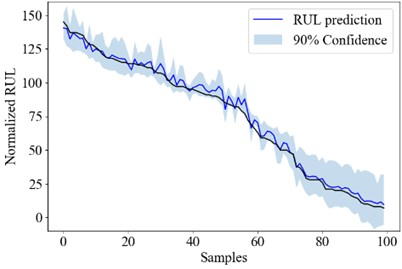
a) PT-LSTM

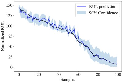
b) PT-CNN

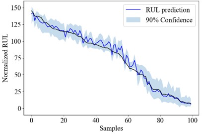
c) PT-SAE

Fig. 2 shows the RUL uncertainty quantification result of each engine in test_FD001 using the PT-LSTM, the PT-CNN and the PT-SAE model. The engine numbers are sorted according to its RUL for better demonstration.

4.4. Result analysis

With PT-BDL model constructed, the data from test_FD001 is used for performance evaluation. Firstly, the data from test_FD001 is normalized with the same scale in the training dataset train_FD001. Then a sliding window with the same time step and window length as train_FD001 is conducted for data segmentation.

The segmented data are then sent to the trained PT-BDL model for RUL prediction. In order to quantify uncertainty in RUL prediction, every data segment is predicted 100 times to obtain 100 prediction results.

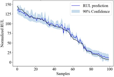
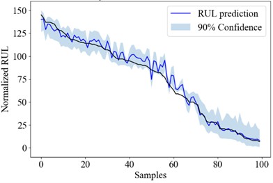
Fig. 3the RUL uncertainty quantification result of Att-ensemble PT-BDL

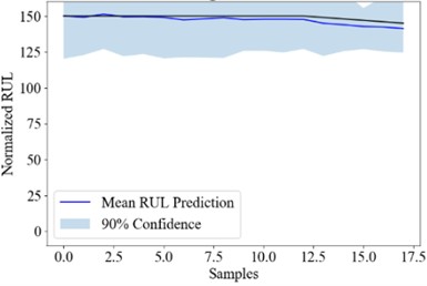
a) #25

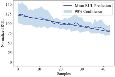
b) #50

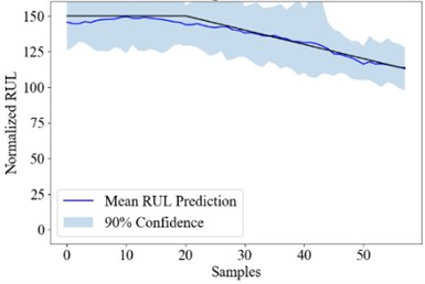
c) #75

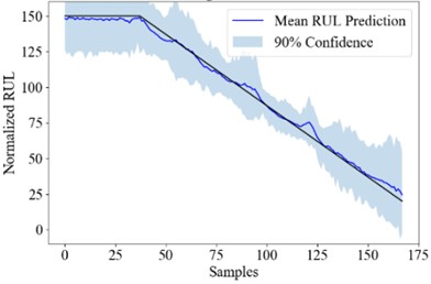
d) #100

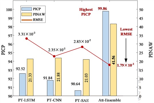
Fig. 3 shows the real RUL (black line), mean predicted RUL (blue line) and 90 % confidence interval (blue area) of engine #25, #50, #75 and #100. The PICP, PINAW and RMSE of the PT-BDL models are calculated and listed in Table 6.

Table 6Prediction performance of the PT-BDL models

PT model	PICP	PINAW	RMSE
PT-LSTM	92.52 %	21.33	3.31×10^-2
PT-CNN	91.84 %	21.88	2.35×10^-2
PT-SAE	90.64 %	21.03	2.83×10^-2
Att-ensemble PT-BDL	99.86 %	41.56	1.79×10^-2

It can be seen from the table that in terms of PICP and RMSE, the PT-BDL model outperforms all of its member algorithms. However, PINAW of the Att-ensemble PT-BDL model is higher than its member algorithms, which is likely because the Bayesian attention-based integration model introduces extra uncertainty into the prediction result.

Fig. 4Prediction performance of the PT-BDL models

4.5. Ablation study and discussion

An ablation study is conducted to further demonstrate the effectiveness of the proposed PT-BDL method. In the ablation study, three Bayesian models with the same structure as PT member algorithms are constructed and trained on subset $Y_{m e m b e r}$ . An Adam optimizer with learning rate set to 1×10^-3 is used for back propagation and the training epoch limitation is 200 epochs.

Fig. 5the RUL uncertainty quantification result of Bayesian models

a) LSTM

b) CNN

c) SAE

Fig. 5 shows the RUL uncertainty quantification result of each engine in test_FD001 using the Bayesian LSTM, Bayesian CNN and Bayesian SAE model. The engine numbers are sorted according to its RUL for better demonstration.

The ability to quantify RUL uncertainty is further evaluated from three aspects, which are PICP, PINAW and RMSE, and the evaluation result is shown in Table 7.

The prediction performance of the PT-BDL models are compared with that of the BDL models and the result is shown in Table 8.

Table 7Prediction performance of the BDL models

Source model	PICP	PINAW	RMSE
Bayesian LSTM	88.28 %	21.52	3.58×10^-2
Bayesian CNN	86.83 %	20.35	3.58×10^-2
Bayesian SAE	86.41 %	21.90	3.99×10^-2
Bayesian ensemble	96.28 %	40.45	2.76×10^-2

Table 8Comparison between the PT-BDL models and the BDL models

	LSTM		CNN		SAE		Ensemble
	BDL	PT-BDL	BDL	PT-BDL	BDL	PT-BDL	BDL	PT-BDL
PICP	88.28 %	92.52 %	86.83 %	91.84 %	86.41 %	90.64 %	96.28 %	99.86 %
PINAW	21.52	21.33	20.35	21.88	21.90	21.03	40.45	41.56
RMSE	3.58×10^-2	3.31×10^-2	3.58×10^-2	2.35×10^-2	3.99×10^-2	2.83×10^-2	2.76×10^-2	1.79×10^-2

It can be seen that PT member algorithm models and PT-BDL models have obvious improvements in PICP and RMSE, which are 4.24 %, 5.01 %, 4.23 % and 3.62 % in PICP and 0.41×10^-², 1.23×10^-2, 1.16×10^-2 and 0.97×10^-2 in RMSE. It proves through transferring parameters in point estimation models to BDL models and attention-based ensemble, the Att-ensemble PT-BDL model can achieve better prediction and uncertainty quantification performance.

5. Conclusions

In this study, an attention-based ensemble method with partial-transfer Bayesian deep learning is proposed for RUL uncertainty quantification under data inefficiency. In the proposed method, well-trained point estimation model is used as source model, of which parameters are transferred to BDL models with the same structure. The transferred parameters in the BDL models are frozen while the other trainable parameters are trained with insufficient data. The trained BDL models are used as member algorithms to construct the attention-based Bayesian model, which integrate BDL models for RUL prediction and uncertainty quantification.

A case study is conducted on the C-MAPSS dataset FD001 to prove the effectiveness of the proposed Att-ensemble PT-BDL method. The train_FD001 dataset is divided into three subsets, of which one subset is used for member algorithm training and another subset is used for integration algorithm training. The trained PT-BDL model is test with test_FD001 and evaluated in terms of PICP, PINAW and RMSE. The results shows that the proposed att-ensemble PT-BDL method exhibited an overall PICP of 99.86 %, an overall PINAW of 41.56 and a RMSE of 1.79×10^-2. The Att-ensemble PT-BDL method outperforms its PT-BDL member algorithms and Bayesian ensemble method in PIC-P and RMSE, proving the effectiveness of both partial transfer method and attention-based ensemble method.

In this study, freeze-tuning instead of full-tuning is chosen mainly based on two specific features:

(1) The scenario of the source model (predicting RUL of aircraft engines) is highly similar to the scenario of the target model (predicting uncertain RUL of aircraft engines).

(2) The training dataset of the target model is rather small (only a small part of the dataset train_FD001).

If the study is under a more universal condition where the training data of the target model is sufficient or the scenario of the target model is different from the scenario of the source model, fine-tuning will be the better choice to achieve partial transfer learning.

The RUL uncertainty in engineering and other practical scenarios are often in the form of asymmetric distribution (namely lognormal distributional etc.) instead of symmetric distribution. In this study, the prior distribution in Bayesian model are set to normal distribution in order to simplify the calculation. In the future work, a more realistic distribution will be used as the prior distribution.

References

J. Gao, Y. Wang, and Z. Sun, “An interpretable RUL prediction method of aircraft engines under complex operating conditions using spatio-temporal features,” Measurement Science and Technology, Vol. 35, No. 7, p. 076003, Jul. 2024, https://doi.org/10.1088/1361-6501/ad3b2c

Publisher
A. Ramachadran et al., “Review of contemporary methods for reliability analysis in aircraft components,” Journal of Aerospace Information Systems, Vol. 21, No. 6, pp. 482–488, Jun. 2024, https://doi.org/10.2514/1.i011277

Publisher
L. Wang, “Predictive maintenance scheduling for aircraft engines based on remaining useful life prediction.,” IEEE Internet of Things Journal, Vol. 11, No. 13, pp. 23020–23031, 2024, https://doi.org/jiot.2024.3376715

Publisher
L. Lin, J. Wu, S. Fu, S. Zhang, C. Tong, and L. Zu, “Channel attention and temporal attention based temporal convolutional network: A dual attention framework for remaining useful life prediction of the aircraft engines,” Advanced Engineering Informatics, Vol. 60, p. 102372, Apr. 2024, https://doi.org/10.1016/j.aei.2024.102372

Publisher
S. Szrama and T. Lodygowski, “Aircraft engine remaining useful life prediction using neural networks and real-life engine operational data,” Advances in Engineering Software, Vol. 192, p. 103645, Jun. 2024, https://doi.org/10.1016/j.advengsoft.2024.103645

Publisher
Y. Keshun, Q. Guangqi, and G. Yingkui, “A 3-D attention-enhanced hybrid neural network for turbofan engine remaining life prediction using CNN and BiLSTM models,” IEEE Sensors Journal, Vol. 24, No. 14, pp. 21893–21905, Jul. 2024, https://doi.org/10.1109/jsen.2023.3296670

Publisher
S. Chen, J. He, P. Wen, J. Zhang, D. Huang, and S. Zhao, “Remaining useful life prognostics and uncertainty quantification for aircraft engines based on convolutional Bayesian long short-term memory neural network,” in Prognostics and Health Management Conference (PHM), pp. 238–244, May 2023, https://doi.org/10.1109/phm58589.2023.00052

Publisher
J. Zhang, J. Tian, P. Yan, S. Wu, H. Luo, and S. Yin, “Multi-hop graph pooling adversarial network for cross-domain remaining useful life prediction: A distributed federated learning perspective,” Reliability Engineering and System Safety, Vol. 244, p. 109950, Apr. 2024, https://doi.org/10.1016/j.ress.2024.109950

Publisher
J. Pearl, Probabilistic Reasoning in Intelligent Systems: Networks of Plausible Inference. Elsevier, 2014.

Search CrossRef
H. Wang and D.-Y. Yeung, “A survey on bayesian deep learning,” ACM Computing Surveys, Vol. 53, No. 5, pp. 1–37, Sep. 2021, https://doi.org/10.1145/3409383

Publisher
Y. Cheng, J. Qv, K. Feng, and T. Han, “A Bayesian adversarial probsparse Transformer model for long-term remaining useful life prediction,” Reliability Engineering and System Safety, Vol. 248, p. 110188, Aug. 2024, https://doi.org/10.1016/j.ress.2024.110188

Publisher
M. Jiang, T. Xing, E. Zio, and X. Zhu, “A Bayesian data-driven framework for aleatoric and epistemic uncertainty quantification in remaining useful life predictions,” IEEE Sensors Journal, Vol. 24, No. 24, pp. 42255–42267, Dec. 2024, https://doi.org/10.1109/jsen.2024.3479079

Publisher
C.-Y. Zhu, Z.-A. Li, X.-W. Dong, M. Wang, and W.-K. Li, “Adaptive optimization deep neural network framework of reliability estimation for engineering structures,” Structures, Vol. 64, p. 106621, Jun. 2024, https://doi.org/10.1016/j.istruc.2024.106621

Publisher
Z. Li, K. Goebel, and D. Wu, “Degradation modeling and remaining useful life prediction of aircraft engines using ensemble learning,” Journal of Engineering for Gas Turbines and Power, Vol. 141, No. 4, Apr. 2019, https://doi.org/10.1115/1.4041674

Publisher
C. Ordóñez, F. Sánchez Lasheras, J. Roca-Pardiñas, and F. J. C. Juez, “A hybrid ARIMA-SVM model for the study of the remaining useful life of aircraft engines,” Journal of Computational and Applied Mathematics, Vol. 346, pp. 184–191, Jan. 2019, https://doi.org/10.1016/j.cam.2018.07.008

Publisher
S. K. Singh, S. Kumar, and J. P. Dwivedi, “A novel soft computing method for engine RUL prediction,” Multimedia Tools and Applications, Vol. 78, No. 4, pp. 4065–4087, Sep. 2017, https://doi.org/10.1007/s11042-017-5204-x

Publisher
I. Remadna, S. L. Terrissa, R. Zemouri, S. Ayad, and N. Zerhouni, “Leveraging the power of the combination of CNN and Bi-directional LSTM networks for aircraft engine RUL estimation,” in 2020 Prognostics and Health Management Conference (PHM-Besançon), pp. 116–121, May 2020, https://doi.org/10.1109/phm-besancon49106.2020.00025

Publisher
Y. Song, G. Shi, L. Chen, X. Huang, and T. Xia, “Remaining useful life prediction of turbofan engine using hybrid model based on autoencoder and bidirectional long short-term memory,” Journal of Shanghai Jiaotong University (Science), Vol. 23, No. S1, pp. 85–94, Dec. 2018, https://doi.org/10.1007/s12204-018-2027-5

Publisher
T. Xia, Y. Song, Y. Zheng, E. Pan, and L. Xi, “An ensemble framework based on convolutional bi-directional LSTM with multiple time windows for remaining useful life estimation,” Computers in Industry, Vol. 115, p. 103182, Feb. 2020, https://doi.org/10.1016/j.compind.2019.103182

Publisher
T. Bayes, “An essay towards solving a problem in the doctrine of chances,” Biometrika, Vol. 45, No. 3-4, pp. 296–315, 1958.

Publisher
A. Kendall and Y. Gal, “What uncertainties do we need in Bayesian deep learning for computer vision?,” in Advances in Neural Information Processing Systems, 2017.

Search CrossRef
K. Weiss, T. M. Khoshgoftaar, and D. Wang, “A survey of transfer learning,” Journal of Big Data, Vol. 3, No. 1, May 2016, https://doi.org/10.1186/s40537-016-0043-6

Publisher
S. J. Pan and Q. Yang, “A survey on transfer learning,” IEEE Transactions on Knowledge and Data Engineering, Vol. 22, No. 10, pp. 1345–1359, Oct. 2010, https://doi.org/10.1109/tkde.2009.191

Publisher
V. Mnih et al., “Recurrent models of visual attention,” in Advances in Neural Information Processing Systems, 2014.

Search CrossRef
D. Bahdanau, K. Cho, and Y. Bengio, “Neural machine translation by jointly learning to align and translate,” arXiv:1409.0473, 2014.

Search CrossRef
T. Xiahou, F. Wang, Y. Liu, and Q. Zhang, “Bayesian dual-input-channel LSTM-based prognostics: toward uncertainty quantification under varying future operations,” IEEE Transactions on Reliability, Vol. 73, No. 1, pp. 328–343, Mar. 2024, https://doi.org/10.1109/tr.2023.3277332

Publisher
Y. Gal and Z. Ghahramani, “Bayesian convolutional neural networks with Bernoulli approximate variational inference,” arXiv:1506.02158, 2015.

Search CrossRef

About this article

Received

January 15, 2026

Accepted

March 12, 2026

Published

April 21, 2026

SUBJECTS

Fault diagnosis based on vibration signal analysis

DOI

https://doi.org/10.21595/jve.2026.26015

Keywords

RUL prediction

uncertainty quantification

attention-based ensemble

transfer learning

Bayesian deep learning

Acknowledgements

Jiyan Zeng and Yaohua Tong contributed equally to this work and should be considered joint first authors. This study was supported by the National Natural Science Foundation of China (Grant No. 52402508), the Aeronautical Science Fund (Grant Nos. 201933051001 and 20240033051001) and the Fundamental Research Funds for the Central Universities, the Research Start-up Funds of Hangzhou International Innovation Institute of Beihang University under Grant No. 2024KQ069/2024KQ035/2024KQ036.

Data Availability

The datasets generated during and/or analyzed during the current study are available from the corresponding author on reasonable request.

Author Contributions

Jiyan Zeng: investigation, methodology, software, writing-original draft. Yaohua Tong: data curation, formal analysis, methodology, software, writing-original draft. Yujie Cheng: conceptualization, supervision, writing-review and editing. Chen Lu: funding acquisition, project administration, supervision.

Conflict of interest

Dr. Chen Lu is an editorial board member for Journal of Vibroengineering and was not involved in the editorial review and/or the decision to publish this article.

This is an open access article distributed under the Creative Commons Attribution License, which permits unrestricted use, distribution, and reproduction in any medium, provided the original work is properly cited.