Abstract
Pipeline magnetic flux leakage inspection, mainly used for pipeline defect detection, is an important means of inner examination technology on pipeline. Flux leakage testing can't obtain valid defect identification signals by one hundred percent because of magnetization of the magnetic leakage field, the measured shape, size and location of pipeline defects, materials and operating conditions, and lift-off value, pole pitch and the length of steel brush during the measurement as well as forged pipe fittings such as welding seam, stiffener, flange and tee on the pipeline to be tested. This article reaches a conclusion that magnetic flux density distribution is influenced by the depth and width of defect through respectively researching magnetic leakage field of individual defect and double defects (thickness type) by finite-element method. It also conducts the numerical analysis on pipeline welding seam, stiffener, flange (increased wall thickness type) and tee (compound) leakage magnetic field in detection conditions of the same direction, and concludes their distribution rules of magnetic flux density. The characteristic parameters of distinguishing defect magnetic flux leakage field and the part of the pipeline magnetic flux leakage, derived from analysis and comparison of results on defective pipeline and conduit joint, stiffener, flange and tee magnetic flux leakage, provide a foundation of qualitative identification for accurately recognizing pipeline defect and eliminating the impact of other ancillary fittings on a pipe on pipeline magnetic flux leakage, and they can also offer infallible data to pipeline maintenance as a basis of quantitative analysis.
1. Introduction
Pipeline magnetic flux leakage inspection is an important means of pipeline defect detection [1]. According to principle of magnetic flux leakage testing, when the tube has defects, magnetic field distribution of defects on both sides will change [2]. The shape, size and location of defects can approximately be tested via change of magnetic flux leakage measured by the hall probe on the detector [3]. But in general, pipeline magnetic flux leakage is signally interfered by magnetization of the leakage field, the measured shape, size and location of pipeline defects, materials and operating conditions, and lift-off value, pole pitch and the length of steel brush during the measurement as well as forged pipe fittings such as welding seam, stiffener, flange and tee on the pipeline to be tested [4]. It can cause negative influences on pipeline magnetic flux leakage testing results, such as errors of measurement, defect misjudge and omission [5].
This situation often occurs in the pipeline internal inspection, resulting in unnecessary panic. For example, in 2004, the test report within some segments, finished by a testing company in the UK with the commission of a pipeline company in China, suggests over 1000 all kinds of defects, in which as many as 68 of them need to be repaired. After excavation and verification, it is found that there are only 9 faults coinciding with testing results, and other 59 ones are mostly caused by signal interference of casing layer, welding seam and stiffener. Such a large number of erroneous judgments have caused a large amount of additional economic losses, and brought about questions and complaints of inside testing technology from pipeline operating unit. Based on these above, the author has gained characteristic parameters of discriminating defect and pipeline components magnetic flux leakage field via analyzing and comparing the magnetic leakage field from pipeline defect, welding seam as well as pipe welds, stiffener, flange and tee [1]. Thus it provides a basis of qualitative identification for accurately recognizing pipeline defect and eliminating the impact of other ancillary fittings on a pipe on pipeline magnetic flux leakage, and also offers infallible data to pipeline maintenance as a basis of quantitative analysis [4].
2. Numerical stimulation of the magnetic leakage field of pipeline containing defects
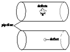
Pipeline defects exist in various forms on the tube [6], with the majority of point-like and pitting corroded defect. When conducting the three-dimensional simulation analysis of pipeline magnetic flux leakage, we usually set up the cone defect model to help with the analysis. We analyze the pipeline magnetic flux leakage under two conditions of single defect as well as adjacent defects according to the characteristics of defects. If no special instructions, all of magnetic flux density curves in the article use the probe detection distance (the same length from the defect center to the sides) as the lateral axis, component of magnetic flux density values as the vertical axis. Pipeline defects all present at the inner face of the pipe, thus called inner pipe defects. The structure is shown in Fig. 1.
Fig. 1Schematic diagram of pipeline defect
2.1. Finite-element analysis of single defect magnetic flux leakage
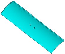
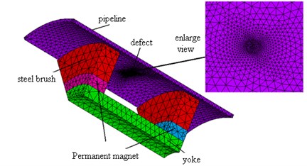
Pipe defect magnetic flux leakage field is influenced by many factors, such as pipeline material, pipeline internal pressure, pipe magnetization, defect size, defect shape and defect location [4]. Among these factors, defect size has the biggest influence on pipe defect magnetic flux leakage signals [7]. Therefore, when analyzing their characteristics, we should first consider the influence of defect size on magnetic leakage signal, and change one of its components to conduct stimulation study. Thus the influence of defect size changing on pipe defect magnetic flux leakage can be judged by researching the radial component BY and the axial component BZ of defect magnetic flux leakage field. The model of finite-element analysis of single defect magnetic flux leakage is shown in Fig. 2.
Fig. 21/8 finite element model of the single defect
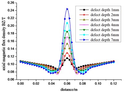
2.1.1. The influence of defect depth change on pipe defect magnetic flux leakage
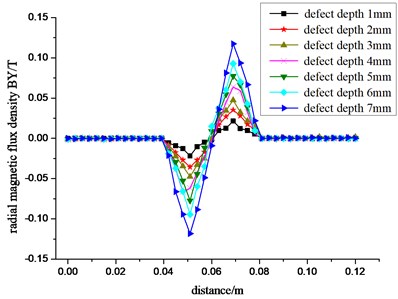
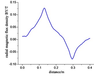
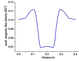
Set conical defect diameter of 10 mm and remain unchanged, change defect depth to respectively 1 mm, 2 mm, 3 mm, 4 mm, 5 mm, 6 mm, 7 mm, stimulate defect size of different depths with ANSYS, and draw radial and axial components of the graph of pipe defect magnetic flux leakage magnetic flux density from the results. Fig. 3 shows the change of the radial component BY and the axial component BZ on defect magnetic flux leakage field with different defect depth.
Fig. 3Change curve of the radial a) and axial b) component of the leakage magnetic field with different depth
a)
b)
Seen from Fig. 3, magnetic flux density components only change nearly defects, and remain slowly placid in the left and the right of defects, which coincides with the signals obtained by the actual sensor. From Fig. 3(a) we know, in single defect of pipeline magnetic flux leakage, radial component BY of magnetic flux density has two peaks of plus and minus. This is because leakage-flux at the edge of defect produces mutation. From the center line of sensing distance namely defect center, BY curve is approximately symmetric, which explains that the signal of magnetic leakage field is nearly the same from both sides of the defect center. There is a zero point of flux-density near the defect center between the plus and the minus which shows there isn`t the radical component signals in defect magnetic flux leakage field. From Fig. 3(b), we know that axial magnetic flux density component BZ of single defect of pipeline magnetic flux leakage only has one positive peak, and from the center line of defect center, BZ curve is approximately bilaterally symmetric. And the displacement is approximately bilaterally equal in relative defect center. It shows that axial magnetic flux leakage signals from both sides of defect center are approximately identical. As the increase of defect depth, peak component of magnetic flux density in magnetic leakage field has a trend of enlargement.
2.1.2. The influence of defects of variations in radius on pipe defect magnetic flux leakage
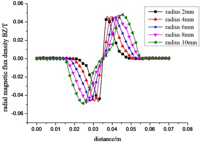
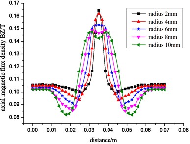
Set up cone defect depth as 3 mm and remain unchanged, change respectively the defect radius to 2 mm, 4 mm, 6 mm, 8 mm, 10 mm, stimulate defect size of different radius by ANSYS, and draw the curve diagram of radial and axial components of pipe defect magnetic flux leakage magnetic flux density, as shown in Fig. 4, respectively.
Seen from Fig. 4, as the increase of defect radius, the radial component BY peak is gradually growing with increasing trend of smaller. On the contrary, the axial component BZ peak is then gradually decreasing, and BY peak is changing from single-peak to peak-to-peak level as the increase of defect radius. The distance between BY two peaks and BZ curve span is progressively widening, which shows that magnetic leakage signal in defect magnetic flux leakage field has positive correlation with defect radius.
Fig. 4Change curve of the radial a) and axial b) component of the leakage magnetic field with different radius
a)
b)
2.2. Finite-element analysis of double magnetic flux leakage
Affected by corrosive media, pipe usually presents the phenomena of multiple adjacent defects and defect even as zone [8]. Pipeline defect recognition can be further improved through researching whether defect magnetic flux leakage fields influence each other or not. Double simulation model of the magnetic leakage field is shown in Fig. 5.
Fig. 51/8 finite element model of the double defect
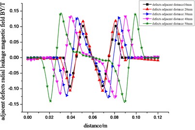
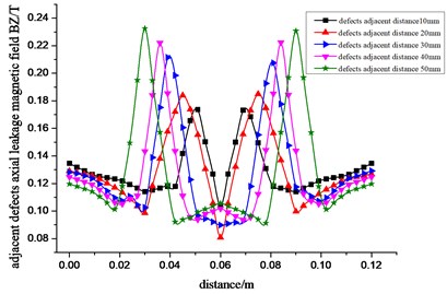
Set up two defects as cone defects, diameter as 10 mm, depth as 4 mm, and analyze the distribution of magnetic leakage field when the adjacent distance of two defects is respectively 10 mm, 20 mm, 30 mm, 40 mm, 50 mm. The results are shown in Fig. 6.
Fig. 6The radial a) and axial b) magnetic flux density distribution curve of the double-defect leakage magnetic field
a)
b)
Seen from Fig. 6, when the adjacent defects exist in the pipeline, radial component BY of magnetic flux density presents four peaks of two positive and two negative, and axial component BZ curve of magnetic flux density presents state of convex with two peaks. From the center line of sensing distance namely center distance of two adjacent defects, BY and BZ curves are approximately symmetric. The nearer two defects are, the more influence they have on each other. With the increase of space, its influence gradually reduces. When the space between two defects is more than 50 mm, its influence can be ignored. And magnetic flux density curves can be divided into two separate curves of magnetic flux leakage of defects.
By comparing to the analysis of single defect and adjacent magnetic leakage field, because of the interaction between adjacent defects, and defects of the same depth and width, peak of magnetic flux density in adjacent defect magnetic leakage field is bigger than that of single defect magnetic flux leakage, namely the adjacent defect magnetic flux leakage causes bigger damage on pipe, more likely causing pipeline accidents.
3. Finite-element analysis of pipe fittings leak magnetic field
When conducting flux leakage testing on pipe, besides the tube defect, forged fittings such as stiffener, welding seam, flange and tee on tube also produce magnetic leakage field, interfering with pipe defect magnetic flux leakage [9]. The following is the Fem Simulative Analysis on stiffener, welding seam, flange and tee.
3.1. Numerical analysis of pipeline stiffener
3.1.1. Finite element analysis model of the pipe body
To reduce the economic costs and rationally use resources, oil pipeline can inevitably be used after being repaired. Finite-element analysis is conducted on reinforcement plate magnetic leakage field by the pipeline base model in order to distinguish defect magnetic flux leakage field and reinforcement plate magnetic leakage field.
Fig. 7Schematic diagram of pipeline reinforcement plate
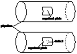
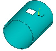
Fig. 8Finite element model of pipeline reinforcement plate
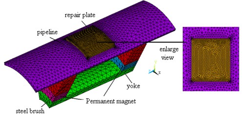
We respectively analyze the pipe with only stiffener as well as with stiffener and defect according to the structure of stiffener. Set up its thickness as constant 5 mm, axial length as variable of 100 mm and 250 mm, the angle along the circumferential direction as 30 degree, its cone defect as 5 mm radius and depth 3 mm. Its structure is shown in Fig. 7 and finite element analysis model shown in Fig. 8.
3.1.2. Finite-element analysis of magnetic flux leakage of pipeline reinforcement plate
3.1.2.1. The influence of axial length of reinforcement plate on magnetic leakage field
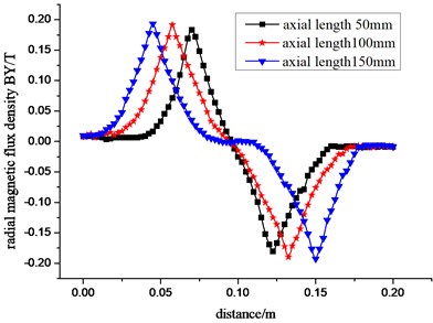
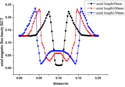
In the actual testing process, axial length of reinforcement plate is the main influential factor to magnetic flux leakage of reinforcement plate. First we analyze the change of magnetic leakage signal resulting from the difference of axial length of reinforcement plate. Set up its thickness as 5 mm, axial length respectively as 50 mm, 100 mm and 150 mm, conduct finite-element analysis on the stiffeners of different sizes to obtain its radial component BY of magnetic flux density and axial component BZ of magnetic flux density, as shown in Fig. 9, respectively.
Fig. 9Change curve of the radial a) and axial b) component of the magnetic density with different length
a)
b)
Seen from Fig. 9, as magnetic Flux leakage testing device getting through reinforcement plate, magnetic leakage field changes significantly. Radial component BY of magnetic flux density has two peaks in plus and minus, and axial component BZ of magnetic flux density also has two peaks in the concave. The value of BY and BZ is approximately symmetric about stiffener center.
With the increase of its axial length, the space of its magnetic flux leakage peak by BY is also gradually growing, nearly equal to its axial length. When the length is more than 100 mm, there is a curve of near straight line in both components of BY and BZ. When the testing direction remains the same, its radial component of magnetic flux density presents first positive peak, then negative peak, while axial magnetic flux density is approximately symmetrical curve of depression, just the opposite of magnetic Flux density distribution in defect magnetic flux leakage field. All of these can be the basis of distinguishing defect magnetic flux leakage field and plate magnetic flux leakage.
3.1.2.2. The influence on magnetic leakage field
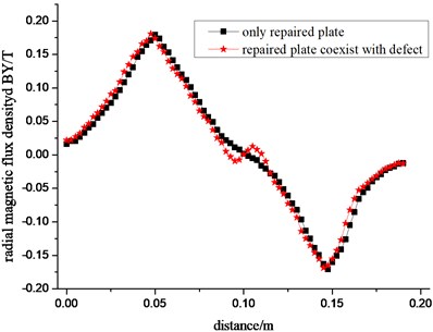
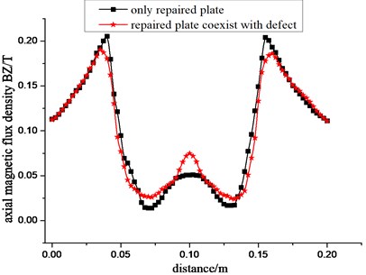
Set up axial length of reinforcement plate as 100 mm, and analyze the magnetic leakage signal under defect-free and defective reinforcement plate (assuming that defects in the central location), as shown in Fig. 10.
From Fig. 10 we know, when pipe has no defects of reinforcement, radial component BY of magnetic leakage field presents two peaks of plus and minus, and the BY value is approximately symmetric about stiffener center. Axial component BZ presents two peaks in concave shape. While pipe has defects of reinforcement, radial component of magnetic flux density has one more two peaks of plus and minus in the defects of stiffener center. There is a convex in concave segments of axial component of magnetic flux density, called the magnetic leakage field. The curve in Fig. 10(a) can be regarded as morphology of magnetic leakage field containing defect pipe reinforcement to correctly judge the real state of the pipe.
Fig. 10The radial a) and axial b) magnetic flux density curve of the leakage magnetic field with reinforcing plate
a)
b)
3.2. Numerical simulation of piping butt weld, flange and tee
3.2.1. Finite element method model of piping butt weld
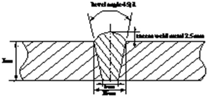
Pipe welding line detecting is a difficult problem in NDT (Non-Destructive Testing). In actual engineering detection [10], testing methods such as ultrasound and -ray are mostly used to detect the defects of bubbles, cracks and inclusions in welding seam. This article uses the circumferential weld of 377 pipeline interfaces as its object of study to analyze distribution of weld leakage magnetic field. According to the requirement of engineering to the up – attachment ring welding seam structure and size, the structure diagram of piping butt weld is established as shown in Fig. 11. Fig. 12 shows finite element analysis model of girth welds.
Fig. 11Schematic diagram of pipe girth butt weld
3.2.2. Flange model of finite element analysis
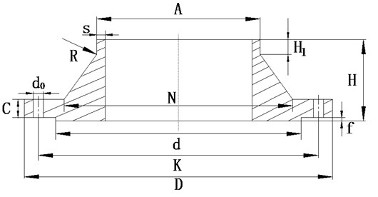
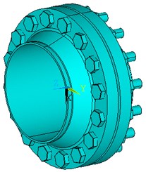
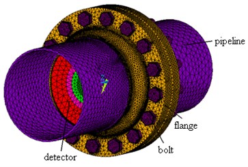
Pipe flange connection generally consists of a set of flanges, bolts, nuts and gaskets, and its usage makes the tube wall increase at junction [11]. So it surely produces magnetic leakage signal as the detector gets through the flange joints, here using HG20592 welding steel flanges. Flange dimensions are shown in Table 1, and its structure shown in Fig. 14.
Table 1Flange size (mm)
Conduit packing DN | Outside diameter | Bolts | ||||||||||||
Quantity | Diameter | |||||||||||||
363 | 377 | 600 | 56 | 522 | 150 | 20 | 442 | 7 | 10 | 425 | 5 | 16 | 39 | 36 |
Fig. 121/8 finite element model of pipe girth butt weld
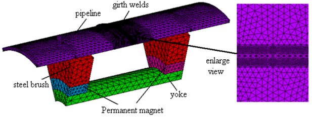
Fig. 13Schematic diagram of flange
This article selects 20# Steel as flange material, 45# Steel as nut and bolt. Magnetization curve of 20# Steel and 45# Steel is looked up from Handbook of commonly used Steels Magnetic Characteristic curve, shown in Figs. 15 and 16. A certain amount of interpolation points on magnetization curve has respective corresponding value of in Table 2 and in Table 3.
Fig. 16 shows the flange models of finite element analysis according to Fig. 13.
Fig. 14B-H curves of 20# steel
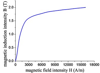
Fig. 15B-H curves of 45# steel
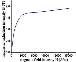
Table 2B/H value of 20# steel
Fit point | (A/m) | (T) | Fit point | (A/m) | (T) |
1 | 0 | 0 | 9 | 7000 | 1.82 |
2 | 400 | 0.25 | 10 | 8000 | 1.85 |
3 | 800 | 0.9 | 11 | 10000 | 1.89 |
4 | 2000 | 1.47 | 12 | 11000 | 1.915 |
5 | 3000 | 1.6 | 13 | 12000 | 1.925 |
6 | 4000 | 1.68 | 14 | 14000 | 1.97 |
7 | 5000 | 1.73 | 15 | 15000 | 1.98 |
8 | 6000 | 1.77 | 16 | 16000 | 2.01 |
Table 3B/H value of 45# steel
Fit point | (A/m) | (T) | Fit point | (A/m) | (T) |
1 | 0 | 0 | 5 | 5000 | 1.73 |
2 | 500 | 0.8 | 6 | 7500 | 1.75 |
3 | 1000 | 1.16 | 7 | 10000 | 1.81 |
4 | 2500 | 1.67 | 8 | 15000 | 1.91 |
Fig. 16The finite element model of flange
3.2.3. Tee models of finite element analysis
Magnetic leakage field from tee is called compound magnetic leakage field. Fig. 18 shows the tee model of magnetic leakage field of finite element analysis according to schematic diagram of tee with pipe connection structure shown in Fig. 17 [12, 13]. The tee uses the rule size correspondent with 377 pipe in the criteria [14, 15]. Its dimensions are shown in Table 4.
Fig. 17Tee schematic diagram
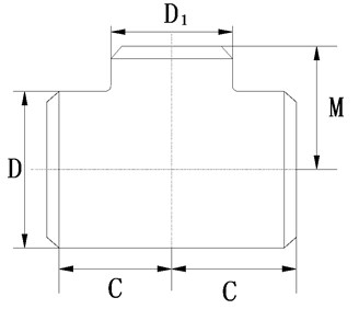
Fig. 18Tees model magnetic leakage field of FEM
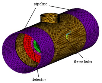
Table 4Tee dimension (mm)
Nominal diameter DN | Slope outside diameter | Center to end | ||
350×350×300 | 377 | 325 | 279 | 270 |
3.2.4. Finite element analysis of welding seam and flange magnetic leakage field
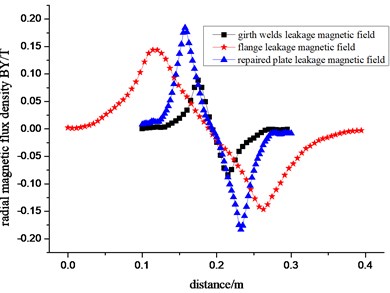
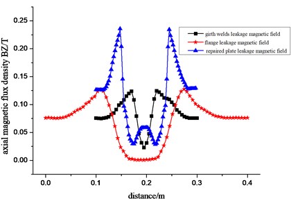
All magnetic leakage field from welding seam, flange and reinforcement plate belong to the magnetic leakage field of the wall thickness increases. Fig. 19 shows the analysis of circumferential weld of pipe and flange leakage magnetic field, as well as the distributing comparison between welding seam, flange and stiffener magnetic leakage field.
Seen from Fig. 19, in cases of the same direction as the magnetic flux leakage testing, there are two peaks in plus and minus in radial component of welding seam, flange and stiffener (increased wall thickness type) in magnetic leakage field, and first comes the positive peak, then the negative peak, with axial component of magnetic flux density for concave shape. While the radial component of magnetic flux density in defect magnetic flux leakage field first presents the negative peak, then the positive peak, with axial component of flux-density for convex shape, which means that magnetic flux density distribution of the two is exactly opposite. The peak value and peak separation are main differences of magnetic flux density curves of welding seam, flange and reinforcement plate, which generally result from geometric sizes of different parts. By the analysis of defect magnetic flux leakage field, we can know that pipeline defect size can be got from the quantitative processing on peak value and peak spacing of magnetic flux density curves, while magnetic flux density distribution of the magnetic leakage field of increased wall thickness is exactly opposite to that of defect magnetic flux leakage field. By the analysis of reinforcement plate magnetic leakage field, we can know that its size can be obtained from the quantitative processing on peak value of magnetic flux density curves and peak spacing. Weld and flange model can be considered as the stiffener model of changing its thickness and width, which means that the geometry of the magnetic flux leakage source in increased wall thickness of the magnetic leakage field can be obtained from the quantitative processing on peak value and peak spacing of magnetic flux density curves. The above shapes can be used as the basis of judging welding seam, flange and reinforcement plate.
Fig. 19Curve of magnetic flux density components radial a) and axial b)
a)
b)
Fig. 20The radial a) and axial b) components of flux-density in tee magnetic field leakage
a)
b)
3.2.5. Finite element analysis of tee leakage magnetic field
Due to the variety of tees, we take the reducing tee of nominal diameter as 350×350×150 for example to conduct the finite-element analysis. When pipeline magnetic flux leakage testing instrument passes through the piping branch junctions, pipes and tees are magnetized by the two-pole, and magnetic line mainly goes through the wall of the tube and tees, while some part of it gets into the air of pole faces through the wall of tees. We extract flux-density of tee magnetic leakage field according to the way of drawing defect magnetic flux leakage field. Figs. 20(a) and 20(b) show respectively the radial and axial components of flux-density in tee magnetic field leakage.
We can know from the overall of Fig. 26 and Fig. 27 that compared with magnetic leakage field of increased wall thickness of magnetic flux leakage source, radial magnetic flux density of tee leakage magnetic field also presents two peaks in plus and minus, with the axial component for concave shape. There is a part concave of the curve remaining generally the same magnetic flux density. The gentle curve represents the magnetic leakage signal caused by sensor getting through the perforation of tee.
4. Comparison of analysis on magnetic leakage field of pipeline defect and pipe fittings
4.1. Comparison of curve peak of magnetic flux density in different magnetic leakage field
From the analysis of pipe defect magnetic flux leakage, the intensity of the field increases with the growing of defect depth. In order to figure out the connection between defect magnetic flux leakage field and the peak value of magnetic leakage field from welding seam, stiffener and pipe fitting, we compare the radial component of magnetic flux density in different depths of defects and the pipe components curves of radial magnetic flux density, as shown in Fig. 21. When the pipe defect gets 7 mm, the wall is penetrated with the through-hole defect, and magnetic flux density component reaches the maximum. Fig. 22 shows the comparison of its peak and that of radial component of magnetic flux density on pipeline components.
Fig. 21Combined curve of radial component of magnetic flux density
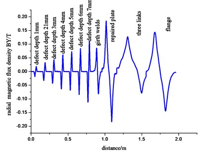
Fig. 22Comprehensive correlation curve of radial magnetic flux density peaks
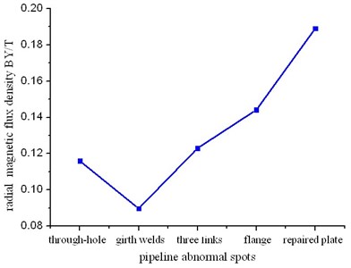
From the overall of Fig. 21 and Fig. 22, only when magnetic flux density peak of pipe welding line is smaller than that of through-hole, the density peaks of pipe stiffener, tee and flange are all bigger than the through-hole peak. Therefore, we can judge the source of leakage according to the peak size of the radial magnetic flux density, that is to say, the peak value of radial component can be used as characteristic parameters to identify magnetic leakage field of the defect and other pipe components. As the radial component peaks of magnetic leakage signal measured actually are more than a certain value, its signal is produced by pipe stiffener or fittings, not by defect magnetic flux leakage signals.
4.2. Comparison of magnetic flux density curve span in different magnetic leakage field
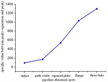
Magnetic flux density curve span is the interval between the positive peak and the negative one in distribution of radial component of magnetic flux density. According to the basic rule of flux leakage testing, magnetic flux can produce mutation at the defect edge or both ends of the other part of pipe, thus producing the magnetic leakage field. The peak of radial component of magnetic flux density on measured pipe presents at both ends of pipe components or pipeline defect, and their widths can be determined by the peak separation. In general, the radius of individual defect is less than the width of stiffener, tee and flange, resulting in that magnetic flux density curve span of single defect magnetic flux leakage is less than that of stiffener, tee and flange. Fig. 23 shows the comparison of peak spans of defect and peak curve in magnetic flux density of fittings and welding seam. Because the widths of defect and weld are similar, magnetic flux density curve span of defect and weld leakage magnetic field are approximate.
In order to further analyze the connection between the peak and span of magnetic flux density curves and defect, welding seam, stiffener, flange as well as tee magnetic leakage field, we can use the ratio of peak spacing of magnetic flux density curve and its peak value to analyze, in which the ratio is specific value of the width and height of the radial component of magnetic flux density curve in pipeline magnetic flux leakage, as shown in Fig. 24. From the comparison we know that the ratio of defect magnetic flux leakage field remains the lowest, while the ratio of stiffener, welding seam, flange and tee magnetic leakage field increases. Therefore the peak span and size of magnetic flux density curves can also be used as characteristic parameter to distinguish the defect and magnetic leakage field of other pipe components.
Fig. 23Comparison of span in radial component of magnetic flux density
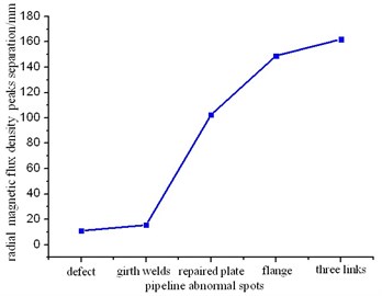
Fig. 24Ratio of peak span and peak value
4.3. Analysis of multi-sensor signals of magnetic flux leakage in different leakage magnetic field
In the actual engineering testing process, the collection of magnetic leakage signal is made of many sensors. With analyzing the measured distribution of magnetic flux leakage pipeline, because the distribution information is influenced by a single sensor institutions and the scope of testing, we cannot get full access to the distribution within pipeline magnetic flux leakage only by a single sensor. Therefore it needs to comprehensively process the information from multiple sensors in order to get the complete evaluation on defect, welding seam, stiffener, flange and tee magnetic leakage field.
From the structure of welding seam and flange, they form uniform distribution along the pipeline, causing its magnetic leakage signal to be evenly distributed along the pipeline. During the testing, all the sensors in testing devices can detect the magnetic leakage signal from them, and theoretically each of sensors gets the same signal, which reveals the essential difference between the distributions of defects, stiffener and tee magnetic leakage field and welding seam and flange leakage magnetic field. The small size of single defect leads to the small span and peak value of magnetic leakage signal. So there are only some of sensors which can detect the magnetic leakage signal from single defect. Because the size of stiffener and tee is bigger than single defect, numbers of sensors measured from reinforcement plate and tee are more than that from defect magnetic flux leakage signals. We can also determine the source of magnetic leakage field on the basis of number of measured magnetic flux leakage signal of the sensor, which can also used as characteristic parameter to identify defects and magnetic leakage field of other pipe fittings.
5. Conclusions
This article uses finite-element analysis to obtain the differences between the distribution rule of pipeline defect (single and the adjacent defects) magnetic leakage field, welding seam, stiffener, flange and tee magnetic leakage field as well as its distribution of magnetic flux leakage signals, thus reaching the feature parameter of recognizing defects and magnetic leakage signal of pipe fittings. The following are main conclusions:
1) Researching single defect and magnetic leakage field of adjacent defect (thickness type) by finite-element analysis, reaching the influence of defect depth and width on its magnetic flux density distribution. Signal peak of single defect magnetic flux leakage on the pipe is gradually increasing with the growing of defect depth, and radial peak spacing and axial component of the inflection point spacing are gradually increasing with the growing of defect width. The regulation can be the basis of the late identification of defect size. Compared with the radial component of magnetic flux leakage of single defect, that of adjacent defect has more than a positive peak and a negative one, with the axial component being more than a positive peak. Under the same size of defects, magnetic flux density peak of adjacent flaws is bigger than that of single one, which shows that the adjacent defects have more damage to pipe.
2) In the cases of the same direction detection, we conduct the numerical analysis on welding seam, stiffener, flange (Increased wall thickness type) and tee (compound) magnetic leakage field, and compare the results with the distribution of the magnetic leakage flux density to obtain the fact that the order of positive and negative peaks’ appearance in distribution curve of the radial component of magnetic flux density from welding seam, stiffener, flange and tee leakage magnetic field is exactly opposite to the distribution curve of radial magnetic flux density from defect magnetic flux leakage field. Comparing the distribution curve of axial magnetic flux density, magnetic flux density curves of welding seam, reinforcement plate, flange and tee leakage magnetic field present the concave shape. The regularities of distribution can be used as characteristic quantity to distinguish the pipeline defects and fittings for guiding the actual engineering detection.
3) According to comparison and analysis of defect magnetic flux leakage field and welding seam, stiffener, flange and tee leakage magnetic field, we also found that defect magnetic flux leakage field and its unusual location of leakage magnetic field in other parts of pipeline can be differentiated by the peak value of the radial component of magnetic flux leakage signals, the peak spacing as well as the measured number of sensors of magnetic flux leakage signal.
References
-
Li Y., Tian G. Y., Ward S. Numerical simulation on magnetic flux leakage evaluation at high speed. NDT&E International, Vol. 39, Issue 5, 2006, p. 367-373.
-
Joshi A., Udpa L., Udpa S., et al. Adaptive wavelets for characterizing magnetic flux leakage signals from pipeline inspection. IEEE Transactions on Magnetics, Vol. 42, Issue 10, 2006, p. 3168-3170.
-
Bruno A. C., Schifini R., Khüner G. S., et al. New magnetic techniques for inspection and metal-loss assessment of oil pipelines. Journal of Magnetism and Magnetic Materials, Vol. 226, 2001, p. 2061-2062.
-
Hari K. C., Nabi M., Kulkarni S. V. Improved FEM model for defect-shape construction from MFL signal by using genetic algorithm. Science, Measurement and Technology, IET, Vol. 1, Issue 4, 2007 p. 196-200.
-
Atherton D. L. Finite element calculations and computer measurements of magnetic flux leakage patterns for pits. British Journal of Non-Destructive Testing, Vol. 30, Issue 3, 1988, p. 159-162.
-
Amineh R. K., Nikolova N. K., Reilly J. P., et al. Characterization of surface-breaking cracks using one tangential component of magnetic leakage field measurements. IEEE Transactions on Magnetics, Vol. 44, Issue 4, 2008, p. 516-524.
-
Li L. M., Huang S. L., Wang X. F., et al. Stress induced magnetic field abnormality. Transactions of Nonferrous Metals Society of China (English Edition), Vol. 13, Issue 1, 2003, p. 6-9.
-
Krause T. W., Little R. W., Barnes R., et al. Effect of stress concentration on magnetic flux leakage signals from blind-hole defects in stressed pipeline steel. Journal of Research in Nondestructive Evaluation, Vol. 8, Issue 2, 1996, p. 83-100.
-
Jian F., Zhang F. J., Lu S. X., et al. Three-axis magnetic flux leakage in-line inspection simulation based on finite-element analysis. Chinese Physics B, Vol. 22, Issue 1, 2013, p. 018103.
-
Mandayam S., Udpa L., Udpa S. S., et al. Invariance transformations for magnetic flux leakage signals. IEEE Transactions on Magnetics, Vol. 32, Issue 3, 1996, p. 1577-1580.
-
Katoh M., Masumoto N., Nishio K., et al. Modeling of the yoke-magnetization in MFL-testing by finite elements. NDT&E International, Vol. 36, Issue 7, 2003, p. 479-486.
-
Chen L., Que P., Huang Z., et al. Three-dimensional finite element analysis of magnetic flux leakage signals caused by transmission pipeline complex corrosion. Journal of the Japan Petroleum Institute, Vol. 48, Issue 5, 2005, p. 314-318.
-
Lord W., Wang J. H. Defect characterization for magnetic leakage fields. British Journal of NDT, Vol. 19, Issue 1, 1997, p. 14-18.
-
Nestleroth J. B., Bubenik T. A. Magnetic Flux Leakage (MFL) Technology for Natural Gas Pipeline Inspection. Battelle, Report Number GRI-00/0180 to the Gas Research Institute, 1999.
-
Tamburrino A., Ventre S., Rubinacci G. Reconstruction techniques for electrical resistance tomography. IEEE Transactions on Magnetics, Vol. 36, Issue 4, 2000, p. 1132-1135.
About this article

