Research on 3D MFL testing of wire rope based on empirical wavelet transform and SRCNN

Chen, Qihang; Zhang, Juwei; Li, Bing

doi:10.21595/jve.2022.22267

Journal of Vibroengineering

Browse Journal

Submit article

Published: 30 June 2022

Check for updates

Research on 3D MFL testing of wire rope based on empirical wavelet transform and SRCNN

Qihang Chen¹

Juwei Zhang²

Bing Li³

^{1, 2, 3}Electrical Engineering College, Henan University of Science and Technology, Luoyang, China

^{1, 2, 3}Henan Province New Energy Vehicle Power Electronics and Power Transmission Engineering Research Center, Henan University of Science and Technology, Luoyang, China

Corresponding Author:

Bing Li

Cite the article Download PDF

Downloads 656

WoS Core Citations 1

CrossRef Citations 2

Abstract

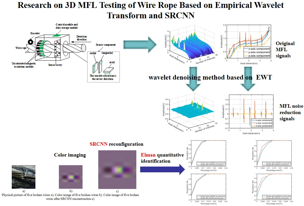
Magnetic flux leakage (MFL) testing is one of the most effective methods in nondestructive testing of wire rope. However, traditional MFL testing devices have problems such as low recognition rate, single detection dimension and fuzzy magnetic leakage image. Based on the non-saturated magnetic excitation 3D MFL testing device, this paper proposes a wavelet denoising method based on empirical wavelet transform (EWT) to denoise the collected 3D MFL signal. After noise reduction, the Signal-to-Noise Ratio (SNR) and Root Mean Squared Error (RMSE) of the three dimensions have improved. Color imaging technology is used to fuse defect grayscale images into color images, and Super-Resolution Convolutional Neural Network (SRCNN) is applied to MFL images of broken wires. After SRCNN reconstruction, the resolution of defect color images is improved. The color moment feature of the defect color image is extracted as the input of the Elman neural network to quantitatively identify broken wires. Experimental results show that the noise reduction algorithm can effectively suppress the noise in three dimensions, and the broken wires recognition rate after reconstruction has been significantly improved, which verifies the effectiveness of SRCNN in wire rope MFL images.

Research on 3D MFL testing of wire rope based on empirical wavelet transform and SRCNN

Highlights

The wavelet filtering algorithm based on EWT is used to denoise the 3D MFL data, which improves the SNR of the 3D MFL signal and reduces the RMSE.
Using the method of combining color imaging and SRCNN, the grayscale image is fused into a color image. At the same time, the resolution is improved after reconstruction by SRCNN, and more edge information is obtained.
The color moment features of the color images before and after reconstruction by SRCNN are extracted as the input of Elman neural network, and the results show that the image recognition rate after reconstruction is significantly improved.

1. Introduction

Wire rope has the advantages of high strength, good elasticity, and strong carrying capacity, and is widely used in coal, mines, cable cars and other fields. As a load-bearing component, wire rope will have fatigue, wear or even fracture due to various reasons during service. Its load-bearing capacity and remaining life are directly related to the safety of production equipment and personnel [1]. Therefore, it is very important to detect the damage of the wire rope. The existing testing methods include ultrasonic, infrared, radiographic and electromagnetic testing technologies. Among them, electromagnetic testing is widely used in nondestructive testing of wire rope due to its low cost, simple principle, and suitable for wire rope with complex structures but good magnetic conductivity. Electromagnetic testing includes magnetic flux leakage (MFL), eddy current testing, and metal magnetic memory (MMM) testing. The principle of the MFL testing technology is to apply a magnetic field to the surface of the wire rope, when there are defects in the wire rope, the permeability of the defects changes, and the magnetic field signal leaks into the air. The magnetic sensor detects the leakage magnetic field and analyzes the collected signal to determine whether the component has defects, and then quantitatively identify the defects [2].

In the design of MFL testing device, common sensors include induction coils, hall sensors, giant magneto resistance (GMR) sensors, tunnel magneto resistance (TMR) sensors, and so on. The improved magnetic field detection sensors can detect wire rope damage more effectively, so many scholars have done a lot of designs in this regard. Zhao et al. [3] designed a wire rope nondestructive detection system composed of 30 hall sensor array, the system realizes the accurate axial positioning and circumferential distribution of defects, and effectively overcomes the influence of traditional induction coil detection on the speed of wire rope movement. Zhang et al. [4] designed the GMR sensor array to be evenly distributed on the circumference of the wire rope to collect the wire rope radial MFL signal. Zhang [5] proposed a small excitation system that uses a small-volume hall sensor element to form a sensor array to obtain MFL signals on the wire rope surface. Compared with the traditional device, the device is small in size and it weighs only 508 g. Although the existing devices can better detect the MFL signal of the wire rope, most of them only collect the signal of the radial or the radial and axial components of the leakage magnetic field. In fact, the spatial MFL signal has three components: axial component, radial component and tangential component. Each component carries a lot of defect summary information. Dutta [6] showed through simulation and analysis that the tangential flux leakage element is indeed a potential key part of the MFL test. Peng [7] designed a 3D MFL testing device using TMR sensor, which can simultaneously collect component information in three dimensions: axial, radial and tangential. Compared with a one-dimensional acquisition device, this device can collect more dimensional information, and the recognition rate of three-dimensional components is higher than that of single-dimensional component.

After the magnetic sensor obtains the leakage magnetic field on the surface of the wire rope, it uses signal processing and image processing technology to reduce the noise of the collected signal. Since the MFL signal on the surface of the wire rope contains a lot of noise, the noise reduction algorithm used directly affects the damage identification of the wire rope. Wavelet is the most commonly used method in the application of MFL signals, such as wavelet multi-resolution analysis [8], wavelet threshold [9], wavelet denoising based on compressed sensing [4], etc. Tan [4] used the compressed sensing wavelet filter algorithm to reduce the noise of the MFL signal, and verified the superiority of the proposed noise reduction algorithm in suppressing high-frequency noise, and achieved good recognition results. Kim and Park [10] used Hilbert transform to process the signal to obtain the signal envelope. This algorithm is simple and effective, but the denoising effect is average. Qiao [11] adopted the improved EEMD noise reduction algorithm to reduce the noise of the magnetic memory signal of the mine wire rope, but the denoising effect is not obvious, and the SNR is only slightly improved.

Image processing technology can visualize the MFL signal of the defect, improve the quality and resolution of the image, and is of great significance to the quantitative analysis of the defect. Tan [12] adopted the SR reconstruction method based on Tikhonov regularization to enhance the defect grayscale image and increase the resolution of the magnetic field grayscale image by 3 times. Li [13] used a super-resolution algorithm based on interpolation, using Non-Subsampled Shear Wave Transform (NSST) combined with Principal Component Analysis (PCA) and Gaussian Fuzzy Logic (GFL) to improve the resolution and quality of grayscale images. Although these methods improve the image quality, the processing result is still grayscale. The amount of information contained in the grayscale image is too small, and it is not easy to quantitatively identify the defect image. Zheng [14] performed pseudo-color image processing on the MFL image of the wire rope, so that the generated image can show subtle differences that were difficult to detect in the previous grayscale image. But the image effect of small broken wires is not obvious.

Aiming at the problems of the existing MFL testing device with single dimension, low SNR after denoising, and inconspicuous MFL image. A non-saturated magnetic excitation 3D MFL testing device was designed [7], using wavelet denoising method based on EWT to denoise the collected MFL signal. Compared with the wavelet filtering algorithm and the EEMD algorithm, it improves the SNR of the 3D magnetic leakage signal and reduces the RMSE. The cubic spline interpolation method is used to interpolate the perimeter of the 3D MFL data, and the gray level is normalized. Using the method of combining color imaging and SRCNN, the grayscale image is fused into a higher-resolution color image. Extract the color moment features of the color image before and after SRCNN reconstruction as the input of the Elman neural network. By comparing the broken wires recognition rate, it verifies the feasibility and effectiveness of Elman neural network and SRCNN in the broken wires recognition.

2. MFL data collection

This article uses the non-saturated magnetic excitation 3D MFL testing device in Reference [7]. The schematic diagram of the acquisition device is shown in Fig. 1. The device includes a magnetization device, a magnetic sensor array, a control board and a data storage module.

Fig. 1Schematic diagram of 3D MFL signals acquisition device

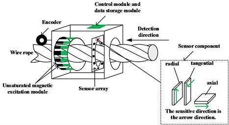
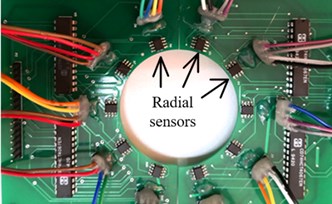
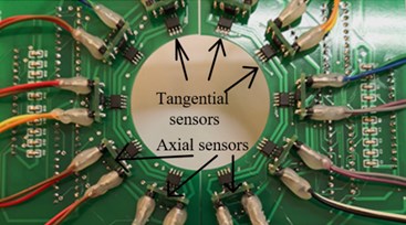
The magnetization device is composed of 12 Nd-Fe-B permanent magnets, which are evenly distributed on the circumference of the wire rope as a non-saturated magnetic excitation source. The residual magnetism of each permanent magnet is 1.18T. The magnetization device can effectively suppress the interference of the external magnetic field and excite the wire rope more uniformly and fully. The data collection process is as follows: push the testing device along the defective wire rope, every time the collection device moves 0.31 meters, the encoder sends out 1024 sampling pulses at equal intervals, and the magnetic sensor array converts the collected MFL signals into voltage signals and stores them in the SD card of the data storage module. The front of the designed 3D MFL signals acquisition board is shown in Fig. 2(a), radial sensors are distributed to collect radial component signals. Fig. 2(b) is the back of the 3D MFL signals acquisition board, with tangential sensors and axial sensors distributed, which are used to collect tangential component signals and axial component signals, respectively. Due to size limitations, the number of sensors in each direction is set to 10, they are distributed in the same circumferential position, and the sensitive directions are perpendicular to each other.

Fig. 2a) 3D MFL signals acquisition board front side, b) reverse side

a)

b)

3. Data processing

Six different broken wires are artificially manufactured for a wire rope in advance, with a total of eight defects. The detection length of the wire rope is 3.8 meters, the diameter is 28 mm, and the distance between the permanent magnet and the wire rope is 15 mm to ensure the same magnetization effect of the wire rope in different dimensions. Push the acquisition device along the wire rope detection direction, the collected original data is shown in Fig. 3(a). The original data contains a lot of noise, these noises mainly include oil pollution on the surface of the wire rope; uneven excitation; the influence of the earth’s magnetic field; strand noise caused by the winding of the wire rope, etc. Each channel is extracted from the axial ( $x$ -axis), radial ( $y$ -axis), and tangential ( $z$ -axis) components respectively, and the original single-channel signal is obtained as shown in Fig. 3(b). The location, size and number of defects cannot be judged from the original data. In order to achieve noise reduction, this paper proposes the wavelet denoising method based on EWT. The processing flow used is shown in Fig. 4, including digital signal processing and image super-resolution reconstruction.

Fig. 3a) Original 3D MFL signals, b) single-channel MFL signals of X-axis, Y-axis and Z-axis components

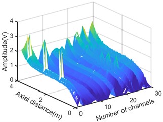
a)

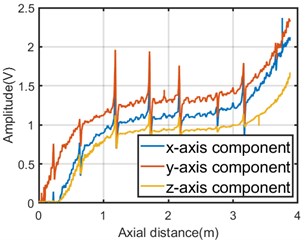
b)

Fig. 43D MFL signals processing flowchart

3.1. EWT theory

Gilles proposed a new signal processing method in 2013 – “Empirical Wavelet Transform”. EWT constructs a set of filters by adaptively segmenting the Fourier spectrum of the signal, and decomposes the signal into a series of AM-FM components arranged from high to low frequencies, thereby extracting feature quantities. EWT avoids the problems of excessive decomposed modal components in EEMD and the need for a large number of iterative operations during extraction. At present, EWT has been initially used in seismic signal processing [15], mechanical fault detection [16], power system signal analysis [17] and other fields.

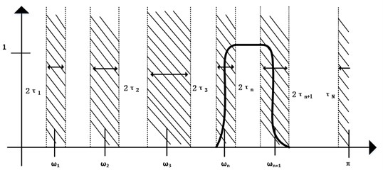
Take real signals as an example. Their frequency spectrum is symmetrical about frequency $ω =$ 0. A normalized Fourier coordinate system with a period of 2 $π$ is established. The research range is $ω \in (0, π)$ , assuming Fourier definition The domain [0, $π$ ] is divided into $N$ continuous partitions, and $ω_{n}$ is used to represent the demarcation bandwidth between each partition ( $ω_{0} =$ 0, $ω_{n} = π$ ). As shown in the fig below, each partition is expressed as $\land_{n} = [ω_{n} - 1, ω_{n}]$ , where a transition section (width 2 $τ n$ ) is defined around each $ω_{n}$ , $τ_{n} = γ ω_{n}$ , and $γ$ is the coefficient. The specific division is shown in Fig. 5.

After determining the segmentation interval $\land_{n}$ , add a wavelet window to it. According to the Meyer wavelet construction method, Gilles defines the empirical scale function and empirical wavelet function [18].

The detail coefficients are generated by empirical wavelet function and signal inner product:

1

W_{f}^{ε} (n, t) = ⟨f, ψ_{n}⟩ = \int f (τ) \bar{ψ_{n} (τ - t)} d τ = F^{- 1} [f (ω) {\hat{ψ}}_{n} (ω)] .

The approximate coefficients are generated by the scaling function and the inner product of the signal:

2

W_{f}^{ε} (0, t) = ⟨f, φ_{1}⟩ = \int f (τ) \bar{φ_{1} (τ - t)} d τ = F^{- 1} [f (ω) {\hat{φ}}_{1} (ω)],

where $ψ_{n} (t)$ and $φ_{1} (t)$ are the empirical wavelet function and scaling function, respectively, ${\hat{ψ}}_{n} (ω)$ and ${\hat{φ}}_{1} (ω)$ are the Fourier transform of $ψ_{n} (t)$ and $φ_{1} (t)$ , $\bar{ψ_{n} (t)}$ and $\bar{φ_{1} (t)}$ denote the complex conjugate of $ψ_{n} (t)$ and $φ_{1} (t)$ , respectively. The original signal is reconstructed as follows:

3

f (t) = w_{f}^{e} (0, t) * φ_{1} (t) + \sum_{n = 1}^{N} w_{f}^{e} (n, t) * ψ_{n} (t) = F^{- 1} [{\hat{w}}_{f}^{e} (0, ω) {\hat{φ}}_{1} (ω)] + \sum_{n = 1}^{N} {\hat{w}}_{f}^{e} (n, ω) * {\hat{ψ}}_{n} (ω) .

The empirical mode $f_{k} (t)$ is defined as follows:

4

f_{0} (t) = w_{f}^{e} (0, t) * φ_{1} (t),

5

f_{k} (t) = w_{f}^{e} (k, t) * ψ_{k} (t) .

Fig. 5Fourier spectrum segmentation diagram

3.2. Wavelet analysis algorithm

Wavelet analysis is an effective signal transformation analysis method developed on the basis of Fourier. Compared with the Fourier transform can only be applied to the decomposition of stationary signals, Wavelet analysis is a partial analysis of the time and frequency of the signal. Through multi-scale subdivision of the signal, it finally achieves the time subdivision at the high frequency and the frequency subdivision at the low frequency.

In order to achieve fast decomposition, Mallat [19] proposed a fast signal decomposition process that expresses non-stationary signals as the expansion of the basis wavelet function and an algorithm that restores and reconstructs the decomposed signal, which is called Mallat algorithm. In the Mallat algorithm, the signal decomposition process in the form of coefficients is as follows:

6

\{\begin{matrix} a_{j + 1} (k) = \sum_{n = - \infty}^{\infty} a_{j} (n) h_{0} (n - 2 k) = a_{j} (k) * {\bar{h}}_{0} (2 k), \\ d_{j + 1} (k) = \sum_{n = - \infty}^{\infty} a_{j} (n) h_{1} (n - 2 k) = a_{j} (k) * {\bar{h}}_{1} (2 k), \end{matrix}

7

a_{j} (k) = \sum_{n = - \infty}^{\infty} a_{j + 1} (n) h_{0} (k - 2 n) + \sum_{n = - \infty}^{\infty} d_{j + 1} (n) h_{1} (k - 2 n) .

Among them, $\bar{h} (k) = h (- k)$ , $h_{0}$ is a low-pass filter, h₁ is a high-pass filter, Eq. (8) is the decomposition formula of Mallat algorithm, Mallat algorithm can separate the signal into multi-resolution. Eq. (9) is the signal reconstruction formula.

3.3. Algorithm description

Using the characteristics of EWT algorithm in the signal spectrum adaptive division and high time-frequency resolution, the wavelet soft threshold and median filtering are combined in the EWT algorithm. Median filtering is to replace the value of a certain point in the sequence with the median value of each point in a neighborhood of the point, which can protect the edge of the signal from blurring, thereby eliminating isolated noise points [20], the noise reduction algorithm steps are as follows:

Step 1: Select the leakage magnetic field data on the surface of the $i$ channel wire rope, $i =$ 1:30.

(1) The signal is Fourier transformed to obtain the frequency spectrum $F (ω)$ , and the frequency spectrum is represented in the scale space.

(2) Calculate the threshold $T$ , and use the threshold T to select the smallest frequency in the scale space as the boundary frequency division of the spectrum.

(3) Construct $N$ empirical wavelets ${\hat{ψ}}_{n} (ω)$ according to the boundary probability.

(4) Use the inverse Fourier transform calculation to obtain the AM-FM modal component of the signal.

Step 2: Select useful AM-FM modal components in the signal, and use wavelet soft threshold to denoise, using db2 wavelet basis to decompose the modal components in 7 layers.

Step 3: Wavelet reconstruction obtains the signal modal component after noise reduction.

Step 4: Perform inverse EWT on the processed signal modal components to obtain noise reduction data.

Step 5: Perform median filtering to make filtering smoother.

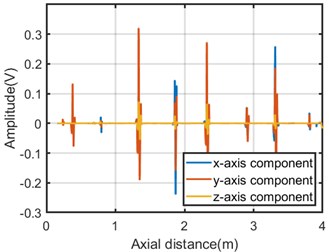
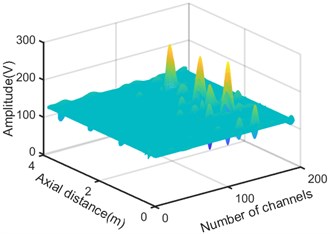
The original data is processed through the algorithm, and the 3D MFL image after noise reduction is shown in Fig. 6(a). Compared with the image before noise reduction, the data after noise reduction reduces the interference of noise, and more obvious defect signals can be observed. From the x-axis in the Fig. 6(a), it is obvious that the defects are mainly around channel 24. This is mainly because the defect is set on the same straight line and the sensor numbers in the three dimensions above the defect are 23, 24, and 25. The approximate position of the defect can be judged through the y-axis, so as to realize the positioning of the defect. Fig. 6(b) shows the single-channel MFL signal of the axial, radial, and tangential components after noise reduction. Not only can the size of the defect be roughly judged by the amplitude, but also the location of the defect can be realized based on the x-axis, and it can be clearly judged that there are roughly 8 broken wires of different sizes on the wire rope. Compared with the original data, it has been significantly improved.

Fig. 6a) 3D MFL signals after noise reduction, b) single-channel MFL signal of X-axis, Y-axis, Z-axis components after noise reduction

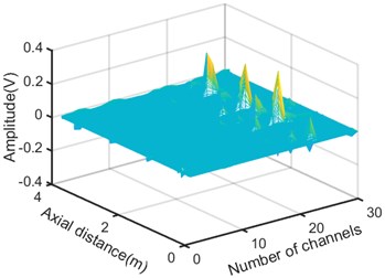
a)

b)

In order to verify the effectiveness of the algorithm, the results calculated in this paper are compared with the wavelet filtering algorithm and the EEMD algorithm. Both the wavelet filtering algorithm and the EEMD algorithm are common and effective noise reduction algorithms. The superiority of the noise reduction algorithm used in this paper is verified by calculating the SNR and the RMSE of the axial, radial and tangential components. The SNR calculation formula is defined as follows:

8

S N R = 10 l g (\sum_{i = 1}^{N} \frac{s^{2} (i)}{\sum_{i = 1}^{N} {(s (i) - \hat{s} (i))}^{2}}),

where $N$ is the number of axial sampling points, $s (i)$ is the MFL signal after noise reduction, and $\hat{s} (i)$ is the effective MFL signal after noise reduction. The higher the SNR, the better the noise reduction effect. The root mean square error is defined as follows:

9

R M S E = \sqrt{\frac{(a (i) - b (i))^{2}}{n}} .

Among them, $a (i)$ represents the noisy signal for which the RMSE value needs to be calculated, and $b (i)$ represents the MFL signal after noise reduction. The smaller the RMSE value, the less noise is included. The noise reduction effect is more obvious.

By extracting the MFL data of 7 wire ropes, donising with different algorithms and calculating their SNR and RSME, the average values obtained are shown in Table 1. it can be seen that the mean value of the SNR in the axial, radial, and tangential directions calculated by the algorithm in this paper is significantly higher than other algorithms, and the mean RMSE is smaller than other algorithms. Among them, the SNR of the radial component is the highest among the three directions, indicating that the radial signal is least affected by noise and has the best denoising effect, which is more conducive to defect location and segmentation.

Table 1The average value of SNR and RMSE of several denoising algorithms

Average	Median filtering and wavelet			Wavelet and EEMD			Proposed algorithm
	Axial component (dB)	Radial component (dB)	Tangential component (dB)	Axial component (dB)	Radial component (dB)	Tangential component (dB)	Axial component (dB)	Radial component (dB)	Tangential component (dB)
SNR	20.5150	22.9395	21.1958	14.2070	25.0467	24.5693	32.0441	43.1946	37.3107
RMSE	0.0096	0.0164	0.0231	0.0060	0.0103	0.0127	0.0031	0.0039	0.0063

4. Image processing

In this section, we will use more mature processing techniques in the field of image processing and deep learning to process MFL data and obtain clearer defect images. The image processing introduced in this section includes data normalization, cubic spline interpolation, color imaging, and SRCNN reconstruction.

4.1. Algorithm description

Data normalization is an indispensable part of image processing. MFL information is converted into grayscale images, and the $x$ -axis component, $y$ -axis component, and $z$ -axis component of the MFL signal are sequentially normalized. Take the $y$ -axis component with the best denoising effect as an example, the specific algorithm is as follows:

(1) Find and record the maximum $y_{m a x}$ and minimum $y_{m i n}$ of the $y$ -axis components, and calculate the mean $y_{m e a n}$ of the data.

(2) Normalize the $y$ -axis data, as in Eq. (10):

10

d a t (i, j) = (\frac{d a t a (i, j) - y_{m i n}}{y_{m a x} - y_{m i n}}) \times 255 - y_{m e a n} + 128 .

Among them, data $(i, j)$ is the MFL data value before normalization, and data $(i, j)$ is the normalized MFL data value after removing the mean. The average removal of the $x$ -axis component, $y$ -axis component, and $z$ -axis component of the MFL signal can make the imaging background information basically consistent.

The designed acquisition system uses a 30-channel sensor array with 10 channels in each dimension. Therefore, the circumferential resolution of the MFL image is 10, which is much smaller than the number of axial sampling points. In order to make the MFL data more intuitive, the circumferential resolution of the $x$ -axis component, $y$ -axis component and $z$ -axis component of the MFL signal is interpolated from 10 to 192 using cubic spline interpolation. Compared with Fig. 6(a), Fig. 7 shows the 3D MFL signal after improving the circumferential resolution. It can be seen that the signal after interpolation is smoother than before, and the defects are more obvious.

Fig. 73D MFL signals after interpolation

4.2. Color imaging

The current MFL images mostly use grayscale images, and a clearer and more intuitive display of MFL characteristics can be obtained by performing image enhancement processing on the grayscale images. The human eye can only distinguish dozens of different grays, but it can distinguish hundreds of different colors [21]. Therefore, applying color imaging to the display of MFL images can highlight the subtle differences that are difficult to detect in the grayscale image, thereby improving the ability to distinguish the details of the image. The specific method is as follows:

(1) Map the normalized $x$ -axis component, $y$ -axis component and $z$ -axis component of the normalized MFL signal to three color channels of red, green, and blue to obtain the MFL color image. To make it easier to distinguish defects, set the weight of the green channel to 0.8, and the weight of the red and blue channels to 1.

(2) Using the modulus maximum method, in the first color channel of the MFL image, the MFL data is summed circumferentially and the sequence $d (j)$ is obtained, where $j =$ 1, 2, 3... $N$ , N is the number of sampling points.

(3) Set a threshold, perform threshold processing on the sequence $d (j)$ , keep the larger value in the sequence, set the points smaller than the threshold to 0, and record the sequence number of the local maximum in the sequence.

(4) According to the actual defect width of the wire rope, the axial length of the defect image is about 192 pixels, so the 192×192×3 color defect image segmentation is based on the maximum serial number value.

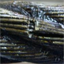
Taking five broken wires as an example, the defect color image obtained according to the above algorithm is shown in Fig. 8(b).

Fig. 8a) Physical picture of five broken wires, b) color image of five broken wires, c) color image of five broken wires after reconstruction

a)

b)

c)

4.3. SRCNN reconstruction

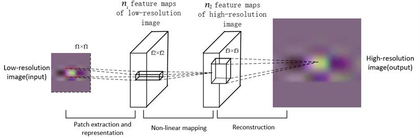
Image super-resolution reconstruction technology uses a group of low-quality, low-resolution images to generate a single high-quality, high-resolution image. This technology can improve the recognition ability and accuracy of the image, and effectively improve the quality of the image. In recent years, deep learning technology has developed rapidly. Dong et al. [22] of the Chinese University of Hong Kong first applied the Convolution Neural Network (CNN) to super-resolution reconstruction in 2016 and proposed a new network SRCNN. Start with the relationship between deep learning and traditional sparse coding (SC), and divide the network into three stages: patch extraction and representation, Non-linear mapping, and reconstruction, make them correspond to the three convolutional layers in the deep convolutional neural network framework, and be unified in the neural network. Thus, super-resolution reconstruction from low-resolution image to high-resolution image is realized. The network directly learns the end-to-end mapping between low-resolution images and high-resolution images. The following is the realization of the SRCNN model [23].

The model consists of three parts. The first part is patch extraction and representation. patch extraction and representation are similar to convolution operations on MFL images through a set of filters. Its first layer is represented as operation $F_{1}$ :

11

F_{1} (Y) = m a x (0, w_{1} * Y + B_{1}) .

The second part is Non-linear mapping. Each n1-dimensional vector obtained in the previous step corresponds to an image block in the original image, and these extracted features are mapped to the n2-dimensional vector. The operation of the second layer is:

12

F_{2} (Y) = m a x (0, w_{2} * F_{1} (Y) + B_{2}) .

The third part is reconstruction, which defines the convolutional layer to generate the final high-resolution image. The operation of the third layer is:

13

F_{3} (Y) = W_{3} * F_{2} (Y) + B_{3} .

Putting the above three operations together form a convolutional neural network, as shown in Fig. 9.

SRCNN is widely used in medical imaging, deep learning and other fields. This is the first time that SRCNN combined with color imaging has been applied to the field of MFL image of wire rope. In this way, 194 MFL images were extracted from different wire ropes with different broken wires and reconstructed by SRCNN. Still taking the five broken wires as the example. Fig. 8(b) and Fig. 8(c) are comparison diagrams of a five broken wires defect before and after SRCNN reconstruction. The defect image has been enlarged from 192×192×3 to 576×576×3. It can be clearly seen from the Fig. 8 that the defect image after SRCNN reconstruction can not only be seen more edge information, and greatly improve the image resolution. Compared with images in other fields, the MFL image itself is blurry and has no particularly significant features. In order to verify the effectiveness of SRCNN, the color moment features of the images before and after reconstruction are selected and used in Elman neural network for broken wire identification.

Fig. 9SRCNN model

4.4. Feature extraction

The color moment feature is proposed by Stricker and Orengo [24]. It is a commonly used color feature and is widely used in the field of image processing. The advantage is that it has the lowest feature vector dimension and lower computational complexity. The distribution of image color information is mainly concentrated in the low-order moments. Using the first-order moment (mean), second-order moment (variance), and third-order moment (skewness) of color information can fully express the color distribution of the image [25]. That is, color characteristics are expressed by color moments. The mathematical model is as follows:

14

μ_{i} = \frac{1}{N} \sum_{j = 1}^{N} P_{i, j},

15

σ_{i} = {(\frac{1}{N} \sum_{j = 1}^{N} (P_{i, j} - μ_{i})^{2})}^{\frac{1}{2}},

16

S_{i} = {(\frac{1}{N} \sum_{j = 1}^{N} (P_{i, j} - μ_{i})^{3})}^{\frac{1}{3}} .

Among them, $P_{i, j}$ represents the probability that a pixel with a gray level of $j$ in the $i$ th color channel component of a color image appears, and $N$ represents the number of pixels in the image. The first three-order color moments of the image $Y$ , $U$ and $V$ , the three components of the image, constitute a 9-dimensional histogram vector, namely, the color features of the image are expressed as follows:

17

F_{c o l o r} = [μ_{Y}, μ_{U}, μ_{V}, σ_{Y}, σ_{U}, σ_{V}, S_{Y}, S_{U}, S_{V}] .

Table 2 lists the characteristic values of the color moments of the six broken wires on the surface of the sample wire rope in this experiment.

Table 2The color moment characteristic values of six broken wires defects

	1 broken wire	2 broken wires	3 broken wires	4 broken wires	5 broken wires	7 broken wires
$μ_{Y}$	127.1759	127.3065	127.3940	127.4200	127.4286	127.3000
$μ_{U}$	102.6897	109.7897	109.2742	102.7000	102,6143	102.4103
$μ_{V}$	128.5655	128.5645	128.5545	128.4533	128.3040	128.1310
$σ_{Y}$	2.7753	3.7131	4.3872	4.6750	5.0467	6.2040
$σ_{U}$	1.2516	2.7310	3.2065	3.5984	3.9340	5.1325
$σ_{V}$	0.5433	2.0646	2.4524	3.6612	4.4231	5.6817
$S_{Y}$	2.6082	2.9757	3.2072	3.3013	3.4444	3.7943
$S_{U}$	1.5168	2.4883	2.6883	2.8462	2.9976	3.3824
$S_{V}$	0.8911	1.9576	2.2305	2.8317	3.1649	3.5840

5. Quantitative identification

Aiming at the problem of slow learning speed of BP neural network algorithm and greater possibility of network training failure, this paper uses Elman neural network to identify defects. Elman neural network is a simple recurrent neural network, proposed by Elman in 1990 [26]. Compared with other feedforward neural networks, the Elman neural network has an additional layer to memorize the output value of the hidden layer neurons at the previous moment, which enhances the global stability of the network. Compared with BP neural network, it has stronger computing power and faster approximation speed, which is more suitable for solving pattern classification problems.

Elman neural network is generally divided into four layers: input layer, hidden layer, receiving layer and output layer. In this paper, a 16× $N$ ×7×7 Elman neural network is designed, and the 9 color moment feature vectors extracted are used as the input of the neural network. $N$ is the number of hidden layers, and both the receiving layer and the output layer are 7.

5.1. Result and analysis

In this experiment, a wire rope with a diameter of 28 mm and a structure of 6×37S+FC was used. In the experiment, broken wires with small spacing are more difficult to identify than broken wires with large spacing, so it is more meaningful to identify broken wires with small spacing. So we obtained 194 samples, including 1, 2, 3, 4, 5, 7 small gaps (about 0.2cm) of broken wires. 135 samples were randomly selected from 194 samples as training samples, and the remaining 59 samples were used as test samples to test the recognition accuracy of the network. In order to verify that the image reconstructed by SRCNN has more edge information and can improve the recognition rate of broken wires, we designed two different types of experiments. In the first group of experiments, 194 samples were reconstructed by SRCNN to extract color moment features, which were trained by Elman neural network. In the second experiment, color moment features were directly extracted from 194 samples and then trained. Elman neural network was used in both experiments, with “tansig” function as the activation function of the hidden layer and “logsig” function as the activation function of the output layer. When $N =$ 5, 10, 15, 20, train the network with training samples, evaluate with test samples, and count the broken wires recognition rate results of each Elman neural network.

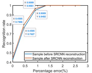
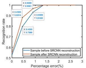
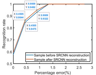
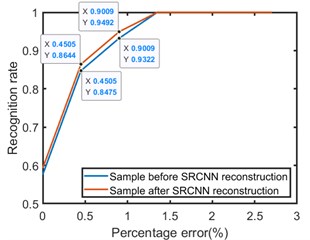
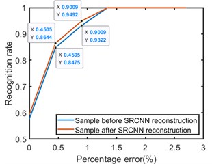
Fig. 10 shows the recognition rate of Elman network with different hidden layer nodes before and after SRCNN reconstruction. It can be seen from the Fig. 10 that the percentage errors of one broken wire and two broken wires are 0.45 % and 0.90 %, respectively, and the maximum error recognition rate is 2.7 %. After SRCNN reconstruction, the recognition rate of one broken wire error and two broken wires error is always higher than before reconstruction. When the percentage errors are 0.45 % and 0.90 %, the recognition rates after reconstruction are 85 % and 96 %, respectively. Among them, when the hidden layer contains 29 nodes, the Elman neural network has the highest recognition rate for broken wires, When the percentage error is 0.90 %, the recognition rate is 98.31 %, the recognition result is shown in Fig. 11.

Fig. 10The recognition effect of different hidden layer nodes before and after SRCNN reconstruction, a) the recognition rate of 5 hidden nodes, b) the recognition rate of 10 hidden nodes, c) the recognition rate of 15 hidden nodes, d) the recognition rate of 20 hidden nodes

The recognition effect of different hidden layer nodes before and after SRCNN reconstruction, a) the recognition rate of 5 hidden nodes, b) the recognition rate of 10 hidden nodes, c) the recognition rate of 15 hidden nodes, d) the recognition rate of 20 hidden nodes

a)

b)

c)

d)

Fig. 11The recognition rate of 29 hidden nodes after SRCNN reconstruction

6. Conclusions

This paper realizes the acquisition and noise reduction of 3D MFL signal of wire rope, as well as the image enhancement and quantitative recognition of broken wires. The selected acquisition device can simultaneously acquire MFL signals in three dimensions of the wire rope. The wavelet denoising method based on EWT is used to denoise the 3D MFL data of the wire rope. Compared with the SNR and RMSE of other filtering algorithms, the superiority of the filtering algorithm in suppressing the MFL noise is verified. The 3D MFL image is mapped to the color space to generate defect color images, and the SRCNN technology is used to reconstruct each defect color image. It solves the problems of low resolution and low recognition rate of traditional MFL grayscale images. The 9 color moments of the reconstructed defective color image are used as the input of the Elman neural network. Compare the broken wire recognition rate of images before and after reconstruction. Experiments show that the recognition rate of the reconstructed image is significantly improved under the error of one broken wire and two broken wires. When the percentage error is 0.90 %, the recognition rate is 98.31 %.

This paper verifies that the application of SRCNN technology in the field of wire rope magnetic flux leakage detection can effectively improve the recognition rate and image quality of broken wires. In the future work, we will study diversified wire rope defect signal collection, optimization of noise reduction algorithm and selection of defect image feature quantity, and use more advanced technologies in the fields of deep learning and artificial neural networks for non-destructive testing of wire ropes.

References

J. Tian, J. Zhou, H. Wang, and G. Meng, “Literature review of research on the technology of wire rope nondestructive inspection in China and abroad,” in MATEC Web of Conferences, Vol. 22, p. 03025, 2015, https://doi.org/10.1051/matecconf/20152203025

Publisher
Y. N. Cao, D. L. Zhang, and D. G. Xun, “The state-of-art of quantitative nondestructive testing of wire ropes,” (in Chinese), Nondestructive Testing, Vol. 27, pp. 91–95, 2005.

Search CrossRef
M. Zhao, D. L. Zhang, and Z. H. Zhou, “The research on quantitative inspection technology to wire rope defect based on hall sensor array,” (in Chinese), Nondestructive Testing, No. 11, pp. 57–60, 2012.

Search CrossRef
J. Zhang and X. Tan, “Quantitative inspection of remanence of broken wire rope based on compressed sensing,” Sensors, Vol. 16, No. 9, p. 1366, Aug. 2016, https://doi.org/10.3390/s16091366

Publisher
D. Zhang, E. Zhang, and S. Pan, “A new signal processing method for the nondestructive testing of a steel wire rope using a small device,” NDT and E International, Vol. 114, p. 102299, Sep. 2020, https://doi.org/10.1016/j.ndteint.2020.102299

Publisher
S. M. Dutta, F. H. Ghorbel, and R. K. Stanley, “Simulation and analysis of 3-D magnetic flux leakage,” IEEE Transactions on Magnetics, Vol. 45, No. 4, pp. 1966–1972, Apr. 2009, https://doi.org/10.1109/tmag.2008.2011896

Publisher
J. Zhang, F. Peng, and J. Chen, “Quantitative detection of wire rope based on three-dimensional magnetic flux leakage color imaging technology,” IEEE Access, Vol. 8, pp. 104165–104174, 2020, https://doi.org/10.1109/access.2020.2999584

Publisher
R. A. Cottis, A. M. Homborg, and J. M. C. Mol, “The relationship between spectral and wavelet techniques for noise analysis,” Electrochimica Acta, Vol. 202, pp. 277–287, Jun. 2016, https://doi.org/10.1016/j.electacta.2015.11.148

Publisher
J. Kwaśniewski, “Application of the wavelet analysis to inspection of compact ropes using a high-efficiency device / Analiza falkowa efektywnym narzędziem diagnostyki lin kompaktowanych,” Archives of Mining Sciences, Vol. 58, No. 1, pp. 159–164, Mar. 2013, https://doi.org/10.2478/amsc-2013-0011

Publisher
J.-W. Kim and S. Park, “Magnetic flux leakage-based local damage detection and quantification for steel wire rope non-destructive evaluation,” Journal of Intelligent Material Systems and Structures, Vol. 29, No. 17, pp. 3396–3410, Oct. 2018, https://doi.org/10.1177/1045389x17721038

Publisher
T. Z. Qiao, Z. X. Li, and B. Q. Jin, “Identification of mining steel rope broken wires based on improved EEMD,” International Journal of Mining and Mineral Engineering, Vol. 7, No. 3, p. 224, 2016, https://doi.org/10.1504/ijmme.2016.078359

Publisher
X. Tan and J. Zhang, “Evaluation of composite wire ropes using unsaturated magnetic excitation and reconstruction image with super-resolution,” Applied Sciences, Vol. 8, No. 5, p. 767, May 2018, https://doi.org/10.3390/app8050767

Publisher
J. Li and J. Zhang, “Quantitative nondestructive testing of wire rope using image super-resolution method and AdaBoost classifier,” Shock and Vibration, Vol. 2019, pp. 1–13, Aug. 2019, https://doi.org/10.1155/2019/1683494

Publisher
P. Zheng and J. Zhang, “Quantitative nondestructive testing of wire rope based on pseudo-color image enhancement technology,” Nondestructive Testing and Evaluation, Vol. 34, No. 3, pp. 221–242, Jul. 2019, https://doi.org/10.1080/10589759.2019.1590827

Publisher
Qin Fabin et al., “Seismic noise suppression based on empirical wavelet transformation,” (in Chinese), China Petroleum Exploration, Vol. 23, No. 5, p. 100, Sep. 2018, https://doi.org/10.3969/j.issn.1672-7703.2018.05.013

Publisher
S. N. Chegini, A. Bagheri, and F. Najafi, “Application of a new EWT-based denoising technique in bearing fault diagnosis,” Measurement, Vol. 144, pp. 275–297, Oct. 2019, https://doi.org/10.1016/j.measurement.2019.05.049

Publisher
K. Thirumala, A. C. Umarikar, and T. Jain, “Estimation of single-phase and three-phase power-quality indices using empirical wavelet transform,” IEEE Transactions on Power Delivery, Vol. 30, No. 1, pp. 445–454, Feb. 2015, https://doi.org/10.1109/tpwrd.2014.2355296

Publisher
J. Gilles, “Empirical wavelet transform,” IEEE Transactions on Signal Processing, Vol. 61, No. 16, pp. 3999–4010, Aug. 2013, https://doi.org/10.1109/tsp.2013.2265222

Publisher
S. Mallat, A Wavelet Tour of Signal Processing. Elsevier, 2009, https://doi.org/10.1016/b978-0-12-374370-1.x0001-8

Publisher
K. Panetta, L. Bao, and S. Agaian, “A new unified impulse noise removal algorithm using a new reference sequence-to-sequence similarity detector,” IEEE Access, Vol. 6, pp. 37225–37236, 2018, https://doi.org/10.1109/access.2018.2850518

Publisher
J. Qu and Y. Du, “Pseudo-color coding based on visual model and perceptual space,” in 2011 International Conference on Control, Automation and Systems Engineering (CASE), Jul. 2011, https://doi.org/10.1109/iccase.2011.5997627

Publisher
C. Dong, C. C. Loy, K. He, and X. Tang, “Image super-resolution using deep convolutional networks,” IEEE Transactions on Pattern Analysis and Machine Intelligence, Vol. 38, No. 2, pp. 295–307, Feb. 2016, https://doi.org/10.1109/tpami.2015.2439281

Publisher
C. Dong, C. C. Loy, K. He, and X. Tang, “Learning a deep convolutional network for image super-resolution,” in Computer Vision – ECCV 2014, pp. 184–199, 2014, https://doi.org/10.1007/978-3-319-10593-2_13

Publisher
M. A. Stricker and M. Orengo, “Similarity of color images,” IS&T/SPIE’s Symposium on Electronic Imaging: Science and Technology, Vol. 2420, p. 381, Mar. 1995, https://doi.org/10.1117/12.205308

Publisher
Z.-C. Huang, P. P. K. Chan, W. W. Y. Ng, and D. S. Yeung, “Content-based image retrieval using color moment and Gabor texture feature,” in 2010 International Conference on Machine Learning and Cybernetics (ICMLC), Jul. 2010, https://doi.org/10.1109/icmlc.2010.5580566

Publisher
J. L. Elman, “Finding structure in time,” Cognitive Science, Vol. 14, No. 2, pp. 179–211, Mar. 1990, https://doi.org/10.1016/0364-0213(90)90002-e

Publisher

Cited by

Research on Quantitative Identification Method for Wire Rope Wire Breakage Damage Signals Based on Multi-Decomposition Information Fusion

(2024)

Detection of Internal Wire Broken in Mining Wire Ropes Based on WOA–VMD and PSO–LSSVM Algorithms

Pengbo Li | Jie Tian | Zeyang Zhou | Wei Wang

(2023)

About this article

Received

20 October 2021

Accepted

30 January 2022

Published

30 June 2022

SUBJECTS

Dynamics and oscillations in electrical and electronics engineering

DOI

https://doi.org/10.21595/jve.2022.22267

Keywords

MFL testing

empirical wavelet transform

SRCNN

Elman neural network

quantitatively identify

Acknowledgements

This work was partially supported by National Natural Science Foundation of China (Grant No. U2004163).

This is an open access article distributed under the Creative Commons Attribution License, which permits unrestricted use, distribution, and reproduction in any medium, provided the original work is properly cited.

Previous article in issue Previous Next article in issue Next

Research article

2023 08 08

Gabor wavelet transform combined with area CNN in appearance intelligent detection of stayed cables

Zhiqiang Li

Research article

2021 02 06

Applying deep learning and wavelet transform for predicting the vibration behavior in variable thickness skew composite plates with intermediate elastic support

Wael A. Altabey

Research article

2019 11 15

Chaotic time series prediction using wavelet transform and multi-model hybrid method

Tian Feng, Shuying Yang, Feng Han

Research article

2019 09 30

Bearing fault diagnosis based on feature extraction of empirical wavelet transform (EWT) and fuzzy logic system (FLS) under variable operating conditions

Fawzi Gougam, Chemseddine Rahmoune, Djamel Benazzouz, Boualem Merainani

Q. Chen, J. Zhang, and B. Li, “Research on 3D MFL testing of wire rope based on empirical wavelet transform and SRCNN,” Journal of Vibroengineering, Vol. 24, No. 4, pp. 779–792, Jun. 2022, https://doi.org/10.21595/jve.2022.22267

Copy Extrica

Copied to clipboard!

TY  - JOUR
DO  - 10.21595/jve.2022.22267
UR  - https://doi.org/10.21595/jve.2022.22267
TI  - Research on 3D MFL testing of wire rope based on empirical wavelet transform and SRCNN
T2  - Journal of Vibroengineering
AU  - Chen, Qihang
AU  - Zhang, Juwei
AU  - Li, Bing
PY  - 2022
DA  - 2022/06/30
PB  - JVE International Ltd.
SP  - 779-792
VL  - 24
IS  - 4
SN  - 1392-8716
SN  - 2538-8460
ER  - 

Copy Ris

Copied to clipboard!

@article{Chen_2022,
	doi = {10.21595/jve.2022.22267},
	url = {https://doi.org/10.21595/jve.2022.22267},
	year = 2022,
	month = {mar},
	publisher = {{JVE} International Ltd.},
	volume = {24},
	number = {4},
	pages = {779--792},
	author = {Qihang Chen and Juwei Zhang and Bing Li},
	title = {Research on 3D {MFL} testing of wire rope based on empirical wavelet transform and {SRCNN}},
	journal = {Journal of Vibroengineering}
}

Copy Bibtex

Copied to clipboard!

[1]Q. Chen, J. Zhang, and B. Li, “Research on 3D MFL testing of wire rope based on empirical wavelet transform and SRCNN,” Journal of Vibroengineering, vol. 24, no. 4, pp. 779–792, Mar. 2022, doi: 10.21595/jve.2022.22267.

Copy IEEE

Copied to clipboard!

Chen, Qihang, Juwei Zhang, and Bing Li. “Research on 3D MFL Testing of Wire Rope Based on Empirical Wavelet Transform and SRCNN.” Journal of Vibroengineering 24, no. 4 (March 16, 2022): 779–92. https://doi.org/10.21595/jve.2022.22267.

Copy Chicago

Copied to clipboard!

Research on 3D MFL testing of wire rope based on empirical wavelet transform and SRCNN

Abstract

Highlights

1. Introduction

2. MFL data collection

3. Data processing

3.1. EWT theory

3.2. Wavelet analysis algorithm

3.3. Algorithm description

4. Image processing

4.1. Algorithm description

4.2. Color imaging

4.3. SRCNN reconstruction

4.4. Feature extraction

5. Quantitative identification

5.1. Result and analysis

6. Conclusions

References

Cited by

About this article

Related Articles