Abstract
For the bionic jumping robot, there is contact force between the foot and the environment inevitably. Bionic jumping robots need to interact with the environment for force/position information in a compliant manner. Therefore, it is necessary to analyze the joint stiffness and foot stiffness of a bionic jumping robot. Based on analyzing the muscle arrangement and flexible jumping movement principle of a dog leg, a kind of musculoskeletal leg driven by pneumatic artificial muscles (PAMs) is presented. The centroid trajectory of the bionic leg is planned for jumping. Each joint stiffness is derived by the joint torque, which is changing with PAM inner pressure and joint angular displacement. On the other hand, joint stiffness can be planned by the foot stiffness. A kind of ellipse stiffness model of foot is proposed by analyzing the foot elastic potential energy caused by the contact force, and each joint stiffness of the bionic leg is calculated by the foot stiffness, which is mapping by the Jacobian matrix. The joint angular stiffness is analyzed by changing the foot stiffness ellipse parameters, and the expected joint stiffness of the bionic leg for jumping is planned based on the foot stiffness model. This study will pay a foundation for controlling the joint stiffness to achieve stable jumping of the bionic leg.
1. Introduction
Legged robots have received extensive attention due to they have the characteristic of various gait modes to achieve better terrain adaptability [1]-[4]. In recent years, legged robot research has evolved from static walking to various dynamic motions such as jumping and running.
PAM is a type of soft actuator, has received considerable attention. PAM has mechanical compliance and exhibits many good characteristics, which is very light, has a high force-to-weight ratio compared with other types of actuators, and it can flexibly comply with outside forces. Because of these above-mentioned properties, PAMs have been employed in various robots, and robots actuated by PAMs can achieve comparatively stable motions.
In order to achieve flexible jumping or running, the joint stiffness of the bionic robot needs to be adjusted or controlled to reduce the impact when the robot landing on the ground. In order to achieve high-speed and high-precision movement of the robot, the position and stiffness of each joint of the bionic robot need to be controlled synchronously [5].
Niiyama et al. [6] developed a musculoskeletal bipedal running robot driven by PAMs, which is named as Athlete robot. The experiment of vertical landing is performed, and it is found that the angle of the stiffness ellipse is a key parameter for fall forward and fall backward of the robot landing. Oshima et al. [7] established a stiffness ellipse model of the robotic arm end, which is driven by six PAMs with a bi-articular muscle. Yokoo et al. [8] studied the stiffness ellipse and came to a conclusions. The movement direction of the robot is possible to be changed by changing the angle of the stiffness ellipse. When there is high friction at the end of the leg and there is no movement, the foot end force can occur in a lower stiffness direction. Nakata et al. [9] demonstrated that the jumping direction of the robot can be changed by adjusting the stiffness ratio between the bi-articular muscle and mono-articular muscle at the hip joint. Kaneko at el. [10] presented bionic leg driven by six PAMs with a bi-articular muscles. The relationship between the ground contact reaction force and the angle of stiffness ellipse was established, and the ground contact reaction force is controlled by the feedforward control. Yasuhiro et al. [11] investigated the joint stiffness of a robot and proposed design procedure based on a reference trajectory and the desired joint stiffness. The stability of the robot and design of the joint stiffness was verified by simulation and experiments with a 1-DOF legged robot. T. Nakamura et al. [12] performed the joint position and stiffness control of a manipulator driven by the artificial muscles for instantaneous loads by using a mechanical equilibrium model. This study revealed that it is effective in constraining the influence of load torque by using estimated stiffness method. Miki K. et al. [13], [14] presented a kind of musculoskeletal quadruped robot. The change-able stiffness property of the bionic body was studied by experiments. When the robot walks, the effect of body stiffness on walking stability and foot contact force was analyzed. Tsujita at el. [15] presented a biped robot driven by PAMs. The effect of joint stiffness on walking stability was analyzed and the relationship between muscle tension and robot performance was studied. An oscillating controller was designed to control the joint stiffness. Lei et al. [16] proposed a kind of foot stiffness model by analyzing the foot elastic potential energy caused by the contact force. The mapping relationship between the joint stiffness matrix and the foot stiffness matrix is obtained by the Jacobian matrix. An antagonistic bionic joint position/stiffness control method based on fuzzy neural network compensation control was presented by Zhu et al. [17], which is obviously better than PID control method.
For the bionic leg driven by PAMs, the joint stiffness characteristics change with the PAM arrangement and inner pressure. Joint stiffness directly affects the jumping performance of bionic legs. In order to achieve the flexibility jumping of bionic leg, it is necessary to plan the joint stiffness in order to achieve the jumping movement. It is worth investigating the stiffness property of the bionic leg for jumping movement.
Based on the design principles of bionics, flexibility and lightweight, a musculoskeletal bionic leg driven by PAMs is presented, which is inspired from the muscles distribution of the biological dog’s leg. Firstly, according to the definition of the joint angular stiffness, each joint stiffness is derived, and the joint angular stiffness for jumping movement of the bionic leg is calculated, which is related with the joint motion parameters, the PAM inner pressure. According to the jumping analysis, the changing range of each joint angular stiffness is determined. Secondly, based on analyzing the elastic potential energy of the foot generated by the contact force from ground, an elliptical model is proposed as the foot stiffness model, and the relationship between the foot stiffness ellipse model and joint stiffness is derived, which is mapped by the Jacques matrix of the bionic leg. Finally, the joint stiffness changing with the parameters of the foot stiffness ellipse is analyzed. Finally, the joint stiffness changing with different parameters of the foot stiffness ellipse were compared and analyzed.
2. Musculoskeletal bionic leg
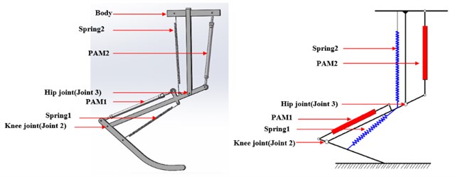
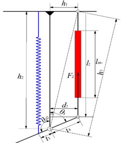
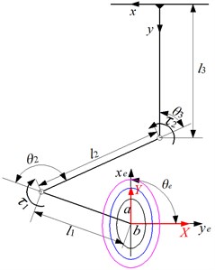
2-DOF musculoskeletal bionic leg is designed, which is inspired by the muscle distribution of dog’s hind limb, as shown in Fig. 1. There are two springs used for slowing down the impact force between the foot and the ground. According to the kinematics of the bionic leg, the rotating range of the knee joint and the hip joint can reach 85° and 55°, respectively.
The jumping movement of the bionic leg is divided into three phases, which are take-off phase, flight phase and landing phase. During the take-off phase, the centroid trajectory of the bionic leg can be planned as a variable quintic polynomial:
where , are the centroid coordinates of the bionic leg along the and direction in the foot-end coordinate system. and are polynomial coefficients. , , (1, 2, 3, 4) are curve tunable parameters, and 3. , are the initial and end time of the flight phase, respectively.
Fig. 1Musculoskeletal bionic leg
According to the motion constraint condition of the centroid, and the value of the adjustable parameters are adjusted, then the centroid trajectory of the bionic leg for jumping movement is derived [18], as shown in Fig. 3, where the blue area is motion space of the bionic leg’s centroid.
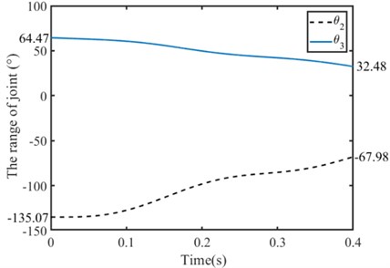
Setting the take-off phase is 0.4 s. According to the kinematics of the bionic leg, the rotating range of each joint can be determined, which should meet the conditions of bionic leg take-off and centroid trajectory planning, as shown in Fig. 3.
Fig. 2Centroid trajectory and centroid motion space
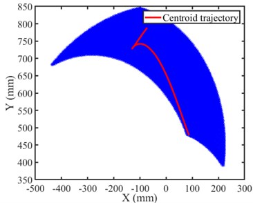
Fig. 3Joint angular displacement during the take-off phase
3. PAM force model
PAM force model describes the relationship between PAM force, inner gas pressure and contraction ratio [19]. According to the Chou model [20], PAM force is:
where is the PAM inner pressure. is the contraction ratio expressed as . is the initial length and is the initial diameter of the PAM. and are constants related to the PAM parameters, , . is the initial braid angle, which is defined as the angle between the PAM axis and each thread of the braided sheath before expansion. For PAM from FESTO company, 30°, 10 mm.
4. Joint angular stiffness
The joint stiffness can be calculated from the joint torque and the joint angular displacement of the bionic leg, which is defined as the partial derivative of joint torque with respect to joint angular displacement [21]:
where is the joint stiffness, is the joint torque, is the joint angular displacement.
4.1. Knee joint
The dynamic motion, such as jumping, landing or running is characterized by large instantaneous forces and short duration. The leg mechanism can be looked as a series manipulator to study the jumping characteristics of the musculoskeletal leg. The musculoskeletal bionic leg is simplified as a 2 DOF mechanism. PAM driving system dynamics is to analyze the relationship between PAM force and the joint driving torque. PAM provide the rotating torque for the joint, as shown in Fig. 4.
Fig. 4Knee joint
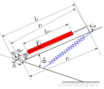
The torque of the knee joint can be calculated. The knee joint torque and PAM driving torque and spring torque :
where is the joint arm length, is the stiffness coefficient of spring 1 and is the change of the knee joint angle.
According to the geometric relationship in Fig. 4, the change of joint angle has little effect on . To simplify, let , the knee stiffness can be calculated as:
where is the PAM1 length. can be derived from the geometric relationship of Fig. 4. can be derived from the Eq. (2). Then the knee joint stiffness change with the PAM inner pressure and the stiffness coefficient is as follows:
The variation range of the angular displacement of the knee joint planned during the take-off process is substituted into the Eq. (5), and the angular stiffness of the knee joint can be calculated.
4.2. Hip joint
The joint torque of the hip joint is shown in Fig. 5.
Fig. 5Hip joint
The relationship between hip joint torque and PAM driving torque and spring torque as follows:
where is the joint arm, is the stiffness coefficient of sprint 2, and is the amount of change in the hip joint angle. From the geometric relationship in Fig. 6, the change of joint angle has little effect on . To simplify the derivation, let , the equation of knee stiffness can be expressed according to Eq. (1) and Eq. (6):
where is the length of the PAM2, can be derived from the geometric relationship of Fig. 6, can be derived from the Eq. (2). Hip stiffness about the inner pressure and the stiffness coefficient is:
The variation range of the angular displacement of the hip joint planned during the take-off process is substituted into Eq. (5) and Eq. (8), joint stiffness can be calculated, which is related to PAM pressure, joint angular displacement, etc.
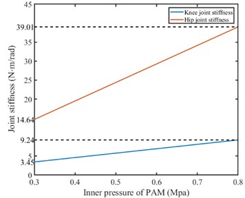
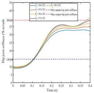
Setting different PAM inner pressure, the knee joint stiffness and the hip joint change with PAM pressure are shown in Fig. 6. In order to achieve jumping movement of the bionic leg, the knee joint stiffness and hip joint stiffness should be within the range of [3.45, 9.24], [14.64, 39.01].
Fig. 6Joint stiffness changing with PAM inner pressure
5. Joint stiffness analysis
5.1. Foot elliptical stiffness model and joint stiffness
The foot stiffness of the bionic leg is set as an elliptical stiffness model [9],[16]. There are there parameters related to the foot stiffness ellipse, which are the long axis length , the short axis length of the ellipse and the ellipse angle . Different foot stiffness ellipse can reflect different foot deformation. One of the stiffness elliptical model is shown in Fig. 7.
Fig. 7Foot stiffness ellipse
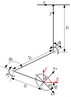
The relationship between the foot stiffness and the joint stiffness can be derived, which is mapped by the bionic leg’s Jacobian matrix. The foot displacement of the bionic leg is:
Then the Jacobian matrix of the bionic leg is:
For 2-DOF bionic leg, a relationship between joint angular displacement and foot displacement can be mapped by the Jacobian matrix of the bionic leg:
where and is the foot displacements along the -axis and -axis direction, respectively. and are the joint angular displacements.
Meanwhile, the relationship between the ground reaction force and the joint driving torque can be expressed by the force Jacobian matrix:
The relationship between the increment of the joint driving torque and the joint angular displacement is as follows:
Based on the relationship between joint torque and joint stiffness, combined with Eq. (11), Eq. (12) and Eq. (13), the relationship between the foot end force and the foot end displacement is derived as following:
Based on the relationship between joint, the expression of the foot stiffness matrix is as follows:
According to the geometric relationship in Fig. 8, the relationship between the deformation of the foot and the elliptical deformation of the stiffness is obtained:
where and are the displacements of the foot displacement in the -axis and -axis directions of the stiffness elliptical coordinate system, respectively.
Considering that the elliptic equation is equal to 1, that is, the elastic energy of the foot end represented by the stiffness elliptic curve is an equipotential energy curve. Set the potential energy value to 1, and the planning of foot stiffness by using these potential energy lines. Based on Eq. (18), the elliptic equation is expressed as follows:
In the foot coordinate system, the foot elastic potential energy can be expressed as follows:
Since the value of the equipotential energy curve is 1, let 1. The expressions of the foot end stiffness can be solved by combining the Eq. (18) and Eq. (19) as follows:
Then the joint stiffness matrix can be derived by Eq. (16) and Eq. (20) as follows:
where:
According to Eq. (13), the joint stiffness of the bionic leg can be obtained from parameter of the foot stiffness ellipse:
where the joint stiffness is a function about the three parameters , , of the foot end stiffness ellipse and the joint angular displacement. The joint angular stiffness of the bionic leg is calculated by changing the parameters of the elliptical stiffness model.
5.2. Calculating results of joint stiffness
5.2.1. Knee joint stiffness
Setting different stiffness ellipse parameters, the joint angular stiffness of the bionic leg is calculated to analyze the relationship between the joint angular stiffness and the foot ellipse parameters. The knee joint stiffness is shown in Fig. 8.
Fig. 8Knee stiffness
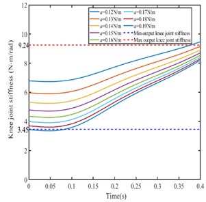
a)0.09 N/m, /2
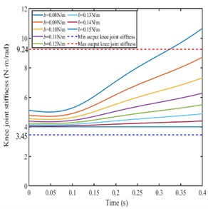
b)0.15 N/m, /2
c)0.15 N/m, 0.09 N/m
Setting the parameters and are constant the parameter is different value, the knee joint stiffness decreases with the parameter increases. According to the knee joint stiffness range in Fig. 7, the changing range of the parameter should be from 0.13 N/m to 0.18 N/m. As shown in Fig. 9(a).
Setting the parameters , are constant and parameter is different value, the knee joint angular stiffness decreases with the parameter increases. According to the knee joint stiffness range in Fig. 7, the changing range of the parameter should be from 0.09 N/m to 0.14 N/m. As shown in Fig. 9(b).
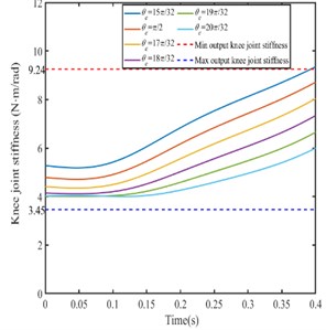
Setting the parameters , are constant and is different value, the knee joint angular stiffness decreases with the parameter increases. According to the knee joint stiffness range in Fig. 7, the changing range of the parameter should be from /2 to 19/32. As shown in Fig. 9(c).
5.2.2. Hip joint stiffness
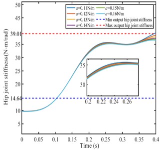
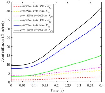
Setting different stiffness ellipse parameters, the hip joint angular stiffness of the bionic leg is calculated to analyze the relationship between the joint angular stiffness and the foot ellipse parameters. The hip joint stiffness is shown in Fig. 9.
As shown in Fig. 9(a), when the parameters and are constant the parameter is set as different value, the hip joint angular stiffness decreases with the parameter increases. According to the hip joint stiffness range in Fig. 7, the changing range of the parameter should be from 0.12 N/m to 0.16 N/m.
As shown in Fig. 9(b), when the parameters , are constant and parameter is set as different value, the hip joint angular stiffness increases with the parameter decreases. According to the hip joint stiffness range in Fig. 7, the changing range of the parameter should be from 0.09 N/m to 0.13 N/m.
As shown in Fig. 9(c), when the parameters , are constant and is set as different value, the hip joint angular stiffness increases with the increases. According to the hip joint stiffness range in Fig. 7, the changing range of the parameter should be from 15/32 to 17/32.
Comparing Fig. 8 and Fig. 9, there are the following conclusions.
When /2 and 0.09 N/m, the range of is from 0.13 N/m to 0.16 N/m, the joint stiffness is in the range of the output joint stiffness.
When 0.15 N/m, /2, the range of is form 0.09 N/m-0.13 N/m, the expected joint stiffness is in the range of the output joint stiffness.
When 0.15 N/m, 0.09 N/m, the range of value of is from /2 to 17/32, the expected joint stiffness is in the range of the output joint stiffness.
Fig. 9Hip stiffness
a)0.09 N/m, /2
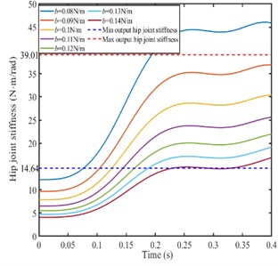
b)0.15 N/m, /2
c)0.15 N/m, 0.09 N/m
5.2.3. Joint stiffness with different ratio of and
Setting the ellipse angle is /2 and different ratio of and , the knee joint stiffness and hip joint stiffness is calculated as shown in Fig. 10.
From Fig. 10(b)-(d), when / is a certain value, the knee joint stiffness and hip joint stiffness increases with the parameters value and decreases, and the increasing trend of hip joint stiffness is larger than that of knee joint. When / changes, the joint stiffness increases with / increases.
Fig. 10Joint stiffness with different parameter ratio of a and b
a) Changing the parameter of the foot stiffness ellipse
b) Joint stiffness (when / = 2)
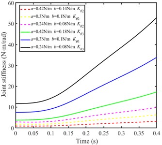
c) Joint stiffness (when / = 3)
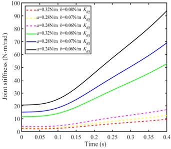
d) Joint stiffness (when / = 4)
6. Foot stiffness with different landing states of bionic leg
Generally, when the line from the centroid of the bionic leg to the foot is perpendicular to the contact surface, the bionic leg can achieve stable landing. So five different landing states are considered for verification, as shown in Fig. 11.
Fig. 11Five landing states of the bionic leg
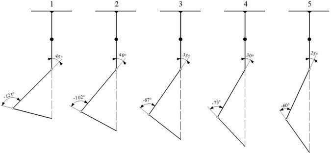
For five different landing states, the knee joint angle is gradually increased and the hip joint is decreased. The corresponding long axis, short axis and ellipse angle of foot stiffness models can be calculated as shown in Table 1.
Table 1Parameters of the foot stiffness ellipse
Leg landing state | (N/m) | (N/m) | (°) |
1 | 34.2161 | 4.3235 | 88.6709 |
2 | 29.2040 | 3.6244 | 89.0048 |
3 | 24.0890 | 2.8715 | 89.2203 |
4 | 18.9009 | 2.0857 | 89.5343 |
5 | 13.6631 | 1.3281 | 89.7150 |
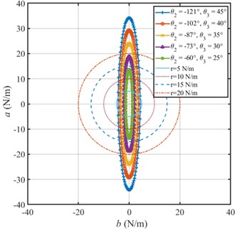
According to the data in Table 1, the foot stiffness ellipse is shown in Fig. 12. For five landing states of bionic leg, the length of the long axis and short axis of the foot stiffness ellipse gradually decrease, and the ellipse angle are close to 90°.
Fig. 12Five kinds of foot stiffness ellipses corresponding to different leg states
7. Conclusions
This study focuses on the joint stiffness planning of a bionic leg driven by PAMs for stable jumping and landing. Firstly, according to the joint angular displacement that can achieve the leg jumping, the changing range of the joint angular stiffness is determined. Secondly, the foot stiffness is planned as an elliptic model, then the relationship between the joint stiffness and the foot stiffness is mapped by the Jacobian matrix of the bionic leg, thus the joint stiffness is calculated by changing the parameters of the foot stiffness elliptic models. Finally, the foot stiffness models of bionic legs with different landing states are calculated, which is to determine the reasonable foot stiffness for stable landing. This study will provide a reference for controlling the joint stiffness to achieve the stable jumping and landing of the bionic leg. The conclusions are drew as follows.
1) For designed bionic leg, the changing range of the joint stiffness is determined for jumping movement. The knee joint stiffness is from 3.45 N⋅m/rad to 9.24 N⋅m/rad, and the hip joint stiffness is from 14.64 N⋅m/rad to 39.01 N⋅m/rad.
2) The foot stiffness has a greater influence on the hip stiffness rather than the knee stiffness. When the parameters of the foot stiffness ellipse / is 4 and the ellipse angle is 90°, the leg can achieve stable jumping.
3) When the ellipse angle is close to 90°, the leg can achieve sable landing.
References
-
L. Ding, “Key technology analysis of BigDog quadruped robot,” Journal of Mechanical Engineering, Vol. 51, No. 7, pp. 1–23, 2015, https://doi.org/10.3901/jme.2015.07.001
-
G. Wang, “The current research status and development strategy on biomimetic robot,” Journal of Mechanical Engineering, Vol. 51, No. 13, pp. 27–44, 2015, https://doi.org/10.3901/jme.2015.13.027
-
H. Ren and J. Fan, “Adaptive backstepping slide mode control of pneumatic position servo system,” Chinese Journal of Mechanical Engineering, Vol. 29, No. 5, pp. 1003–1009, Sep. 2016, https://doi.org/10.3901/cjme.2016.0412.050
-
J. Lei, H. Yu, and T. Wang, “Dynamic bending of bionic flexible body driven by pneumatic artificial muscles (PAMs) for spinning gait of quadruped robot,” Chinese Journal of Mechanical Engineering, Vol. 29, No. 1, pp. 11–20, Jan. 2016, https://doi.org/10.3901/cjme.2015.1016.123
-
J. M. Calderón, W. Moreno, and A. Weitzenfeld, “Fuzzy variable stiffness in landing phase for jumping robot,” in Advances in Intelligent Systems and Computing, Vol. 424, pp. 511–522, 2016, https://doi.org/10.1007/978-3-319-28031-8_45
-
R. Niiyama and Y. Kuniyoshi, “Design principle based on maximum output force profile for a musculoskeletal robot,” Industrial Robot: An International Journal, Vol. 37, No. 3, pp. 250–255, May 2010, https://doi.org/10.1108/01439911011037640
-
Oshima T. and Kumamoto M., “Robot arm constructed with bi-articular muscles,” (in Japanese), Transactions of the Japan Society of Mechanical Engineers, Vol. 61, pp. 4696–4703, 1995.
-
Yokoo T. and Tsuji T., “A tip stiffness control method for robot arm with pneumatic artificial muscles including bi-articular muscles,” (in Japanese), in Technical Meeting on Industrial Instrumentation and Control, pp. 89–94, 2011.
-
Y. Nakata, A. Ide, Y. Nakamura, K. Hirata, and H. Ishiguro, “Hopping of a monopedal robot with a biarticular muscle driven by electromagnetic linear actuators,” in 2012 IEEE International Conference on Robotics and Automation (ICRA), pp. 3153–3160, May 2012, https://doi.org/10.1109/icra.2012.6225362
-
T. Kaneko, K. Ogata, S. Sakaino, and T. Tsuji, “Impact force control based on stiffness ellipse method using biped robot equipped with biarticular muscles,” in 2015 IEEE/RSJ International Conference on Intelligent Robots and Systems (IROS), pp. 2246–2251, Sep. 2015, https://doi.org/10.1109/iros.2015.7353678
-
Y. Sugimoto, D. Nakanishi, M. Nakanishi, and K. Osuka, “Stability and joint stiffness analysis of legged robot’s periodic motion driven by McKibben pneumatic actuator,” Advanced Robotics, Vol. 31, No. 8, pp. 441–452, Apr. 2017, https://doi.org/10.1080/01691864.2016.1273135
-
T. Nakamura, D. Tanaka, and H. Maeda, “Joint stiffness and position control of an artificial muscle manipulator for instantaneous loads using a mechanical equilibrium model,” Advanced Robotics, Vol. 25, No. 3-4, pp. 387–406, Jan. 2011, https://doi.org/10.1163/016918610x552169
-
K. Tsujita and K. Miki, “A study on trunk stiffness and gait stability in quadrupedal locomotion using musculoskeletal robot,” in 15th International Conference on Advanced Robotics, pp. 316–321, 2011.
-
K. Miki and K. Tsujita, “A study of the effect of structural damping on gait stability in quadrupedal locomotion using a musculoskeletal robot,” in 2012 IEEE/RSJ International Conference on Intelligent Robots and Systems (IROS 2012), pp. 1976–1981, Oct. 2012, https://doi.org/10.1109/iros.2012.6386256
-
Tsujita K., Inoura T., Kobayashi T., and Masuda T., “A study on locomotion stability by controling joint stiffness of biped robot with pneumatic actuators,” in Motion and Vibration Control, Springer, 2009, pp. 305–314, https://doi.org/10.1007/978-1-4020-9438-5_30
-
J. Lei, J. Zhu, P. Xie, and M. Tokhi, “Joint variable stiffness of musculoskeletal leg mechanism for quadruped robot,” Advances in Mechanical Engineering, Vol. 9, No. 4, p. 168781401769034, Apr. 2017, https://doi.org/10.1177/1687814017690342
-
J. Zhu, “Position/Stiffness Control of antagonistic bionic joint driven by pneumatic muscles actuators,” Journal of Mechanical Engineering, Vol. 53, No. 13, p. 64, 2017, https://doi.org/10.3901/jme.2017.13.064
-
Chen Z. H., Lei J. T., and Cheng L. Y., “Hopping planning of the bionic leg mechanism driven by PAMs with biarticular muscle,” High Technology Letters, Vol. 25, No. 4, pp. 408–416, 2019, https://doi.org/10.3772/j.issn.1006-6748.2019.04.009
-
D. B. Reynolds, D. W. Repperger, C. A. Phillips, and G. Bandry, “Modeling the dynamic characteristics of pneumatic muscle,” Annals of Biomedical Engineering, Vol. 31, No. 3, pp. 310–317, Mar. 2003, https://doi.org/10.1114/1.1554921
-
Ching-Ping Chou and B. Hannaford, “Measurement and modeling of McKibben pneumatic artificial muscles,” IEEE Transactions on Robotics and Automation, Vol. 12, No. 1, pp. 90–102, 1996, https://doi.org/10.1109/70.481753
-
Xin Wang, Mantian Li, Wei Guo, Pengfei Wang, and Lining Sun, “Development of an antagonistic bionic joint controller for a musculoskeletal quadruped,” in 2013 IEEE/RSJ International Conference on Intelligent Robots and Systems (IROS 2013), pp. 4466–4471, Nov. 2013, https://doi.org/10.1109/iros.2013.6696998
About this article

The authors would like to thank the National Natural Science Foundation of China (Grant No. 51775323).
