Gaussian basis function fitting for stationary solutions of a double-flag hysteretic nonlinear oscillator under colored noise excitation

1. Introduction

Hysteretic nonlinear models have been extensively applied in engineering fields, including mechanical structures, bridge engineering, wing vibrations, magnetic materials, and SMAs. These models effectively describe damping properties in mechanical and bridge systems and material behaviors such as the shape memory effect in SMAs [1-4]. Common mathematical forms include the bilinear model [5], Duhem model [6], Bouc-Wen model [7], and Preisach model [8]. The dynamic response of these models under external excitation holds significant theoretical importance for engineering applications.

Compared to deterministic excitation, random excitation provides a more realistic representation of natural environmental forces. Theoretical methods for analyzing hysteretic nonlinear systems under stochastic excitation have advanced considerably. The equivalent linearization method [9] has been widely applied to study hysteretic models, including the Duhem and bilinear models, under noise excitation [10-12]. The stochastic averaging method, employed by Zhu et al. [7], has also been used to investigate the stochastic dynamics of the Duhem model. Additionally, the Wiener path integral method [13] has been applied to study bilinear [14] and Preisach models [15].

Semi-analytical methods have also gained traction. Guo et al. [16] used exponential closure to fit the steady-state solution of the Fokker-Planck-Kolmogorov (FPK) equation for stochastic vibration systems. Similarly, the system’s response PDF can be approximated using weighted sums of Gaussian basis functions. Due to the radial symmetry of Gaussian functions, this approach is referred to as the radial basis function neural network (RBFNN) method. Researchers have successfully applied this technique to various stochastic nonlinear problems [17-23], demonstrating its accuracy. Chen et al. applied this method on systems excited by the Poisson white noise [19, 20]. Li et al. extended this method to FOPID controller system [21], memristor circuit control [22] and fractional stochastic dynamical systems [23]. Zi Yuan et al. [24] used RBFNN to study a Bouc-Wen model under white noise excitation.

The double-flag hysteretic model is particularly relevant for SMA constitutive modeling. This paper examines its response under Gaussian colored noise, which exhibits temporal decay in autocorrelation and better approximates natural excitations than white noise. The colored noise is treated as white noise filtered through a linear system, allowing the oscillator’s equation of motion to be coupled with the filter equation, forming a three-dimensional Itô stochastic differential system. The GBF fitting method is then applied, minimizing the least-squares error to determine optimal weight coefficients. The method is validated by comparing the fitted steady-state joint PDF, displacement PDF, and velocity PDF with MCS results, confirming its accuracy.

2. Model system

2.1. Mechanical configuration

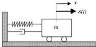
The system under investigation consists of a single-degree-of-freedom oscillator, as illustrated in Fig. 1. The assembly comprises: a mass block ($m$), a linear damper, a shape memory alloy (SMA) spring connected to a rigid support, and the Gaussian colored noise excitation $z\left(t\right)$.

Fig. 1SMA oscillator model

The non-dimensional equation of motion is given by:

1

$\ddot{x}+\mu \dot{x}+F\left(x,\dot{x}\right)=z\left(t\right),$

where $t$ denotes time variable (dots denote time derivatives), $x$ denotes displacement, $\dot{x}$ denotes velocity, $\ddot{x}$ denotes acceleration, $\mu$ denotes linear damping coefficient, and $F\left(x,\dot{x}\right)$denotes displacement-force relationship of the SMA spring. When subjected to loading, a shape memory alloy (SMA) wire undergoes stress-induced martensitic phase transformation. During loading, once the stress reaches a critical threshold, the material exhibits softening behavior characterized by a stress plateau, corresponding to the “yield” segment of the first flag in the double-flag model. Upon unloading, the reverse phase transformation occurs; however, due to the presence of an energy barrier, this process lags behind the decreasing stress, forming another stress plateau that constitutes the second “flag”. This non-coincidence between loading and unloading paths, resulting in a clockwise hysteresis loop, represents the core topological feature of the double-flag model. By employing two back-to-back flag-shaped curves, this model accurately captures the nonlinear stiffness transitions and energy dissipation mechanisms inherent in the phase transformation process of SMA wires, serving as a classic mechanical abstraction for describing such hysteretic behavior.

The colored noise excitation $z\left(t\right)$ is generated by filtering Gaussian white noise through:

2

$\dot{z}=-\lambda z\left(t\right)+\lambda \eta \left(t\right),$

where $\lambda$ is noise delay factor (correlation time), $\eta \left(t\right)$ is Gaussian white noise of intensity $D$, $\left(\eta \right(t)=DdB(t\left)\right)$, where $B\left(t\right)$ denotes the standard Wiener process. The correlation function of the colored noise expressed by Eq. (2) has the form of Eq. (3):

3

$R\left(\tau \right)=E\left[z\left(t\right)z\left(t+\tau \right)\right]=\frac{D}{2}\lambda \mathrm{e}\mathrm{x}\mathrm{p}\left(-\lambda \left|\tau \right|\right).$

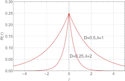
It is obvious that the maximum of the correlation function is $R\left(\tau \right)=\frac{D}{2}\lambda$ and $R\left(\tau \right)$ decreases with the growing delay time $\tau$. Furthermore, the parameter $\lambda$ influence the speed of decrease. The larger the $\lambda$ is, the faster the $R\left(\tau \right)$ decreases. The Fig. 2 shows how the parameter $D$ and $\lambda$ influence the shape of the correlation function. If one wants to study how delay coefficient $\lambda$ impact the system, the product of $D$ and $\lambda$ must be kept as a constant.

Fig. 2Auto-correlation function of the colored noise

2.2. Double-flag model

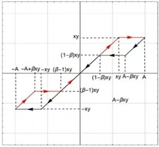
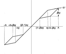
The force-displacement relationship $F\left(x,\dot{x}\right)$ is shown in Fig. 3 Fig. 3(a) shows the linear elastic force $\alpha x$, where $\alpha$ represents the stiffness coefficient. Fig. 3(b) shows the hysteretic force $Z\left(x,\dot{x}\right)$. Combining these gives the flag-shaped restoring force in Fig. 3(c): $F\left(x,\dot{x}\right)=\alpha x+\left(1-\alpha \right)Z$, where, $A$ is the system displacement amplitude, $\beta$ is the energy dissipation coefficient, $x_y$ is the yield displacement.

Fig. 3Double- flag model

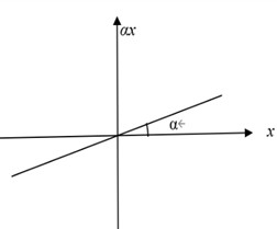
a) Pure elastic response

b) Isolated hysteretic behavior

c) Combined flag-shaped response

The piecewise function for the hysteretic component $Z\left(x,\dot{x}\right)$ is defined separately for loading ($\dot{x}>0$) conditions:

4

$Z=\left\{\begin{array}{ll}x-x_y+A,& -A\le x<-A+\beta x_y,\\ -x_y+\beta x_y,& -A+\beta x_y\le x<-x_y+\beta x_y,\\ x,& -x_y+\beta x_y\le x<x_y,\\ x_y,& x_y\le x\le A,\end{array}\right.$

And unloading conditions ($\dot{x}<0$):

5

$Z=\left\{\begin{array}{ll}-x_y,& -A\le x<-x_y,\\ x,& -x_y\le x<x_y-\beta x_y,\\ x_y-\beta x_y,& x_y-\beta x_y\le x<A-\beta x_y,\\ x+x_y-A,& A-\beta x_y\le x\le A.\end{array}\right.$

The flag hysteresis force can be expressed as Eq. (6) and Eq. (7) in the expression $F\left(x,\dot{x}\right)=\alpha x+(1-\alpha )Z$ shown in Fig. 3(c):

6

$F\left(x,\dot{x}\right)=\left\{\begin{array}{ll}\alpha x+\left(1-\alpha \right)\left(x-x_y+A\right),& -A\le x<-A+\beta x_y,\\ \alpha x+\left(1-\alpha \right)\left(-x_y+\beta x_y\right),& -A+\beta x_y\le x<-x_y+\beta x_y,\\ x,& -x_y+\beta x_y\le x<x_y,\\ \alpha x+\left(1-\alpha \right)x_y,& x_y\le x\le A,\end{array}\right.$

7

$F\left(x，\dot{x}\right)=\left\{\begin{array}{ll}\alpha x-\left(1-\alpha \right)x_y,& -A\le x<-x_y,\\ x,& -x_y\le x<x_y-\beta x_y,\\ \alpha x+\left(1-\alpha \right)\left(x_y-\beta x_y\right),& x_y-\beta x_y\le x<A-\beta x_y,\\ \alpha x+\left(1-\alpha \right)\left(x+x_y-A\right),& A-\beta x_y\le x\le A.\end{array}\right.$

As documented in Ref. [25], previous studies have investigated the response of this double-flag model under Gaussian white noise excitation using the stochastic averaging method. This paper, however, approaches the problem from a different perspective, employing the RBF collocation method.

3. Gaussian basis function fitting

We assume that the approximately stationary PDF of Eq. (10) is $\tilde{P}$, which is in the form of the weighted sum of $N$ Gaussian basis functions:

where, $G\left(\mathbf{r},{\mathbf{\mu }}_{\mathbf{j}},{\sigma }_j\right)$ represents the Gaussian basis function (GBF), $w_j$represents the weight coefficient of the $j$-th GBF, ${\sigma }_j$ represents the standard deviation of the $j$-th GBF, ${\mathbf{r}=\left[x,y,z\right]}^T$ presents the input coordinate vector of the GBF, the vector ${\mathbf{\mu }}_j={\left[{\mu x}_j,{\mu y}_j,{\mu z}_j\right]}^T$ represents the coordinates of the center point of the $j$-th GBF, and $T$ represents the transpose of the matrix:

where $‖r-{\mu }_j‖$ is the Euclidean norm, representing the distance between the input coordinate $r$ and the center point coordinate ${\mu }_j$.

Step 1: construct $N$ Gaussian basis functions. select a domain ${\mathrm{\Omega }}_G=\left[-d_c,d_c\right]\times \left[-d_c,d_c\right]\times \left[-d_c,d_c\right]$ in the $x-y-z\in R^3$ space, then it can be divided into ${N=n}_c\times n_c\times n_c$ grid, each grid point is the center of the GBF. The variance of the basis functions ${\sigma }_{j }$ has a significant impact on the shape. If ${\sigma }_j$ is too large, the shape of each basis function will be too flat; if ${\sigma }_j$ is too small, the shape of the basis functions will be too sharp. When the variance of the basis function is set to ${\sigma }_j=\frac{2d_c}{N}$ (see Ref. [26]) the shape is relatively moderate, where $d_{\mathrm{m}\mathrm{a}\mathrm{x}}$ is the maximum distance between the centers selected by the GBFs.

Step 2: Define the residual $\delta \left(r,w\right)$ function:

Substituting Eq. (11) into Eq. (13), the residual $\delta \left(r,w\right)$ can be rewritten as follows:

where $s_j$ represents the error function, shown as Eq. (15):

The approximation of the PDF function $\tilde{P}$ and the $G_j$ of the GBF function must satisfy the normalization condition for each $j$, that is:

The weight coefficient must have:

Step 3: construct the Lagrange function L(c) by the random sampling method.

In a large enough space ${\mathrm{\Omega }}_S\in R^3$, the defined sampling domain for ${\mathrm{\Omega }}_S=\left[-d_s,d_s\right]\times \left[-d_s,d_s\right]\times \left[-d_s,d_s\right]$, $N_s$ said total sampling points, a suitable $d_s$ should be greater than $d_c$ and less than 2.5 $d_c$, best $N_s$ should choose $N_s=2N$. Define the Lagrange function $L\left(c\right)$ as:

where ${\lambda }^{\text{'}}$ represents the Lagrange multiplier.

The Lagrange multiplier ${\lambda }^{\text{'}}$ and the unknown weight coefficient $w_j$ can be solved through the following two formulas:

The above two equations can be expanded into a matrix form as:

where $k_{mn}=\sum _i^{N_s}{s}_m\left(r_i\right)s_n\left(r_i\right)$, $m,n=\mathrm{1,2},\dots ,N$.

Write Eq. (21) as:

where $A=\left[\begin{array}{cc}\begin{array}{cc}& \\ & \frac{1}{2}K\end{array}& \begin{array}{cc}& 1\\ & ⋮\end{array}\\ \begin{array}{cc}& \\ 0& \cdots \end{array}& \begin{array}{cc}& 1\\ 0& 0\end{array}\end{array}\right]$, $A^T=\left[\begin{array}{cc}\begin{array}{cc}& \\ & \frac{1}{2}K\end{array}& \begin{array}{cc}& 0\\ & ⋮\end{array}\\ \begin{array}{cc}& \\ 1& \cdots \end{array}& \begin{array}{cc}& 0\\ 1& 0\end{array}\end{array}\right]$, $c={[w_1,w_2,\dots ,w_N,{\lambda }^{\text{'}}]}^T\in R^{\left(N+1\right)}$, $b={[\mathrm{0,0},\dots ,1]}^T\in R^{\left(N+1\right)}$.

The error matrix $K$ is expressed as:

Matrix $K$ can also be expressed in the form of matrix multiplication:

where S$=\left[s_{ji}\right]=s_j\left(r_i\right)\in R^{N\times N_s}$.

Finally, the optimal weight coefficient is obtained from Eq. (22):

The first $N$ elemens in vector $C$ are weight coefficients $w_1,w_2,\dots ,w_N$.

After obtaining the fitted approximate probability density, integrating it can yield the joint probability density and the edge probability density:

In this paper, the root mean square error (RMS) of the PDF solution is selected to evaluate the error of GBF fitting:

where $p_i$ and $\stackrel{-}{p_i}$ represent the PDF function evaluated at sample point $x=x_i$ using Monte Carlo simulation (MCS) and GBF fitting methods, respectively.

4. Numerical simulation

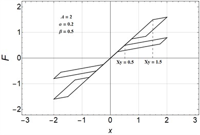
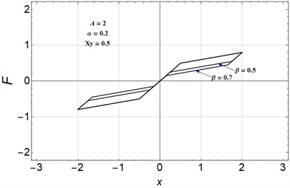
The parameter values are taken as $\alpha =$ 0.2, $A=$ 2, with the damping coefficient$\mu =$ 0.1. When the energy dissipation coefficient $\beta =$ 0.5 is taken and the yield displacement $x_y$ is taken as 0.5 and 1.5 respectively, the double-flag hysteresis curve is shown in Fig. 4(a). When the yield displacement $x_y$ is taken as 0.5, and the energy dissipation coefficients $\beta =$ 0.5 and 0.7 are respectively taken, the double-flag type hysteresis curve is shown in Fig. 4(b).

Fig. 4Double-flag hysteresis plots under different yield displacements

a)

b)

It can be observed from these graphs that when the yield displacement $x_y$ increases from 0.5 to 1.5, the shape of the hysteresis loop undergoes a significant transformation. Furthermore, as the energy dissipation coefficient β increases, the area of the hysteresis loop also increases markedly. These observations indicate that both the yield displacement $x_y$ and the energy dissipation coefficient $\beta$ are critical parameters in determining the area of the double-flag hysteresis loop.

The parameter settings for Gaussian basis function fitting are as follows. First, the computational domain is defined as ${\mathrm{\Omega }}_G=\left[-\mathrm{1,1}\right]\times \left[-\mathrm{1,1}\right]\times \left[-\mathrm{1,1}\right]$ and partitioned into a 25×25×25 grid. Each grid point serves as the center coordinate ${\mu }_j$ of a Gaussian basis function, resulting in a total number of basis functions $N=$25×25×25. Next, the sampling domain is set as ${\mathrm{\Omega }}_{\mathrm{s}}=[-2,\mathrm{ }2]\times [-2,\mathrm{ }2]\times [-2,\mathrm{ }2]$, which is discretized into a finer 50×50×50 grid. The width parameter sigma of the odd basis functions is set equal to the grid spacing/mesh width of the lattice formed by their centers. Each grid point represents a sampling coordinate $r_i$, leading to a total number of sampling points $N_s=$ 50×50×50. These sampling points are sequentially substituted into the error function $s_j\left(r_i\right)$) from Eq. (24), allowing for the construction of matrices S and its transpose $S^T$. Subsequently, matrices $A$ and $A^T$ can be derived based on Eq. (25). Finally, the weight coefficients are computed using Eq. (25).

To verify the accuracy of this method, this paper employs the Monte Carlo simulation (MCS) for validation and utilizes the fourth-order stochastic Runge-Kutta algorithm [27] to generate numerical results. Specifically, 2,000 sets of noise are applied to Eq. (1). Each noise sequence consists of 30,000 data points, among which the last 20,000 points represent stable responses. The simulation time step is set to $∆t=\mathrm{ }$0.005. A total of 2,000×20,000 $\left(x,y\right)$ simulation points are collected to compute the probability of occurrence within each grid cell on the $X$-$Y$ plane. Finally, a comparison is presented between the Gaussian basis function fitting approach and the Monte Carlo simulation results.

4.1. Group one

The fixed parameters were set as $D=$0.005, $\lambda =$5 and $\beta =$ 0.5. Values of $x_y$ = 0.5 and 1.5 were selected to investigate the effect of yield displacement on the steady-state response.

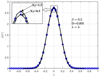
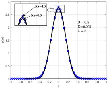
From Fig. 5, it is evident that the joint probability density obtained using the Gaussian basis function (GBF) fitting method and the Monte Carlo simulation (MCS) are in good agreement. Fig. 6 further examines the influence of yield displacement on the steady-state probability density. The results indicate that varying the yield displacement $x_y$ from 0.5 to 1.5 has minimal effect on the steady-state probability density of displacement and velocity. However, as observed in the magnified portion of the figure, a larger yield displacement leads to a slightly higher peak in the probability density distribution. We deem this phenomenon to be reasonable, as higher temperatures lead to larger yield displacements. This consequently causes a slight expansion of the hysteresis loop area and an accompanying increase in energy dissipation, thereby resulting in a correspondingly higher peak in the steady-state probability density.

Fig. 5Joint probability density function under color noise excitation

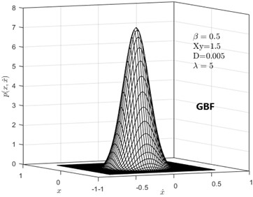
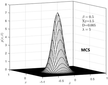
Fig. 6Probability densities: a) p(x) and b) p(y). Solid lines represent GBF, and circles represent MCS

a)

b)

4.2. Group two

The second group of parameters was set to $x_y$= 0.5, and the energy dissipation coefficients $\beta$ were taken as 0.5 and 0.7 respectively to study the effect of the energy dissipation coefficient and compare the influence of the yield displacement and the energy dissipation coefficient on the results.

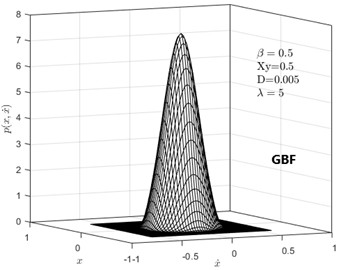
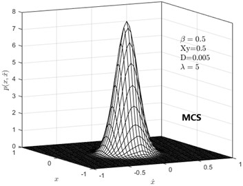
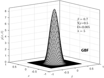
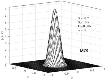
Fig. 7Joint probability density graph when the energy dissipation coefficient takes different values: a) β = 0.5 Gaussian basis function Fitting solution; b) β = 0.5 Monte Carlo simulation; c) β = 0.7 Gaussian basis Function fitting solution; d) β = 0.7 Monte Carlo simulation

a)

b)

c)

d)

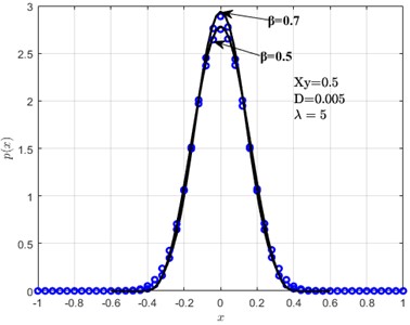
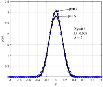
Fig. 8 illustrates that as the energy dissipation coefficient increases, the peak values of the probability density function for displacement and velocity also increase. This phenomenon can be explained as follows: an increased energy dissipation coefficient results in a larger hysteresis loop area, indicating enhanced system damping. Consequently, energy attenuation and vibration amplitude reduction occur. These effects are visually represented in the graph by higher peaks and narrower distribution ranges. A comparison between Fig. 8 and Fig. 6 reveals that the energy dissipation coefficient exerts a more significant influence on the system’s steady-state response than the yield displacement. Generally, for a given SMA wire, the hysteresis loop area in the double-flag model tends to decrease with increasing training cycles. Thus, investigating this area provides an indirect means to assess how training cycles affect the model’s response.

Fig. 8The influence of the energy dissipation coefficient on the probability density of displacement and velocity: a) p(x), b) p(y). Solid line represents GBF, and the circle represents MCS

a)

b)

4.3. Group three

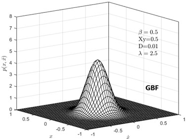
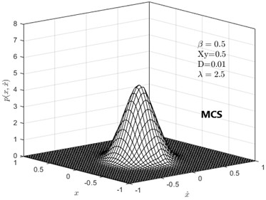
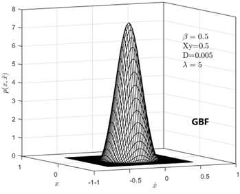
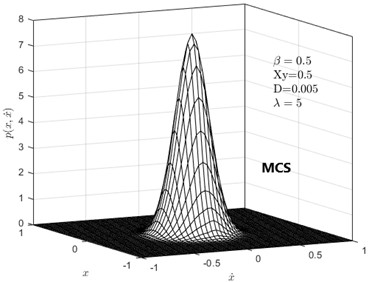
While keeping $\beta$ = 0.5 and $x_y$ = 0.5, both $D$ and $\lambda$ are changed simultaneously, but their product remains unchanged. This is to ensure that the initial cross-correlation function values of the color noise are the same. Take $D=$0.005, $\lambda$= 5 and $D=$0.01, $\lambda$= 2.5. It can be seen from Fig. 2 that the larger the $\lambda$ is, the steeper it decreases with the correlation time. Fig. 9 shows the comparison of the results of the joint probability density under the two noise values.

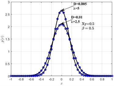
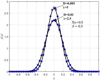
As shown in Fig. 9 and Fig. 10, when $\lambda$ is smaller and $D$ is larger, the response peak becomes lower and the coverage range of the bell-shaped image widens. This suggests that both the vibration amplitude and the velocity distribution interval of the system have expanded. In other words, under the same initial correlation function of colored noise, a higher intensity of white noise passing through the linear filter described by Eq. (2) leads to a stronger system vibration response, which aligns with common physical intuition.

Next, the accuracy of the two algorithms will be compared based on the results presented in this section. The error associated with the GBF method is quantified using Eq. (29), and the corresponding results are summarized in Table 1. Analysis of the data in Table 1 reveals that the root mean square errors across different parameters remain within an acceptable range, thereby validating the effectiveness of the GBF method.

Table 1Root mean square error under different parameters

RMS	$Xy=$ 0.5, $\beta =$ 0.5, $D=$ 0.01, $\lambda =$ 2.5	$Xy=$ 0.5, $\beta =$ 0.5, $D=$ 0.005, $\lambda =$ 5	$Xy=$ 1, $\beta =$ 0.5, $D=$ 0.005, $\lambda =$ 5	$Xy=$ 1.5, $\beta =$ 0.5, $D=$ 0.005, $\lambda =$ 5
RMS-x	0.0085	0.0082	0.0075	0.0089
RMS-y	0.0094	0.0081	0.0091	0.0094

Fig. 9steady-state probability density plots under two noise values: a) and b) are D= 0.01 and λ = 2.5 respectively; c) and d) are D= 0.005 and λ =5 respectively

a)

b)

c)

d)

Fig. 10Probability density function of displacement and velocity under the two noise values

5. Conclusions

This paper investigates the excitation response of a damped vibration system incorporating shape memory alloy (SMA) springs under Gaussian colored noise excitation. The double-flag model was employed to characterize the hysteresis nonlinear behavior of the SMA springs. Using the Gaussian basis function (GBF) fitting method, the joint probability density function, displacement probability density function, and velocity probability density function under various parameter settings were computed. The main conclusions are summarized as follows:

1) The energy dissipation coefficient $\beta$ and the yield displacement $x_y$ are two critical parameters that determine the area of the flag-type hysteresis loop. Since the area enclosed by the hysteresis curve corresponds to the energy dissipated in one loading-unloading cycle, a larger area indicates greater damping capacity. Among these parameters, the energy dissipation coefficient $\beta$ has a more significant influence on the system response compared to the yield displacement $x_y$. As temperature rises, the parent phase of the SMA becomes more stable, requiring higher stress to induce martensite. Consequently, the critical stress increases and the yield displacement $x_y$ shifts to the right. However, it is evident that the yield displacement exerts a relatively minor influence on the system response. In contrast, the number of loading cycles notably affects the area of the hysteresis loop, which in turn has a significant impact on the steady-state response.

2) When other parameters remain constant, a decrease in $\lambda$ combined with an increase in noise intensity D leads to a reduction in peak values, a widening of the coverage range of the probability density function graph, and an expansion of the distribution intervals for both vibration amplitude and velocity.

3) The double-flag model consists of multiple piecewise functions, resulting in numerous non-smooth points-particularly at the junctions between segments-on the hysteresis loop graph. These discontinuities may affect the fitting accuracy of the GBF function.

Theoretically, with a sufficient number of Gaussian basis functions, it is feasible to approximate the solution of the Fokker-Planck-Kolmogorov (FPK) equation with high accuracy. However, due to the three-dimensional nature of the colored noise excitation input variables $(x, y, z)$, constructing a large number of basis functions across all dimensions significantly increases computational complexity, potentially leading to memory overflow. Therefore, this study employs only 25 basis functions in each direction, which allows for acceptable computational accuracy while maintaining manageable computational demands.