The stationary response of piezoelectric cantilever beam model excited by colored noise

1. Introduction

Piezoelectric cantilever model which can transfer the ambient energy into electrical energy has attracted many researchers’ attention in recent decades. The efficiency of the transforming is affected by the piezoelectric cantilever’s response characters. At the beginning of this century, Sndano et.al. [1] and Erturk et.al. [2] designed a type of mono-stable-state piezoelectric cantilever harvester and theoretically predicted the vibrational voltage output. Furthermore, they verified the correctness of this model experimentally. In fact, this type of model only performs large vibration and large voltage output near the fundamental frequency. In other words, when the environmental excitation frequency is far from the fundamental frequency, the voltage output will decrease significantly. After that, scholars extended the piezoelectric harvester model into double well [3-6], triple well [7-9], and even tetradic well [10] models with the help of tip magnet and ancillary repulsive magnets. These structures can improve the efficiency of collecting energy. Scholars also found that potential well as shallow as possible and potential barrier as low as possible will widen the working frequency range. Based on these multi-well models, many dynamical characters such as bifurcation, chaos [8], and randomly chaos [11] are studied sufficiently.

Besides the nonlinear forces induced by repulsive magnets, the nonlinearity of this type of model is caused by two main reasons. The first one is the nonlinear strain-stress relations of the piezoelectric ceramic; the second one is the geometrical nonlinearity of the cantilever’s deformation. Tim Usher et al. [12], Stanton et.al. [13], Angela Triplett et al. [14] and Guo et al. [15] found out that the nonlinear strain-stress relations of piezoelectric ceramic will lead to complex nonlinear dynamical responses even if the cantilever model only has small amplitudes (i.e. the model is under the linear deformation hypothesis). Based on the nonlinear deformation hypothesis, Peyman Firoozy et al. [16] built a new piezoelectric cantilever model, in which he took both the geometrical nonlinearity and the longitudinal inertia nonlinearity into account. Subsequently, the model was quantitatively studied. Some researchers enriched the piezoelectric cantilever study with different academic fields such as aerodynamic and composite material. C. B. Fevzi [17] developed the piezoelectric cantilever with the help of the aerodynamic wing and B. F. C. B. Fevzi [18] and Cakmak et al. [19] deeply investigated the composite beams with different lamination angles.

However, these researches mentioned above are all based on the sinusoidal excitation assumption. Due to the fact that most of the environmental excitations are random, it is very important to extend the research field from deterministic cases into random vibrations. Some researchers used the numerical simulation method to study the mono-stable-state model [20] and multi-stable-state [21, 22] piezoelectric cantilever models which were excited by random excitations. However, more researches about the theoretical prediction of the responses of the randomly excited piezoelectric cantilever harvester model are in need. Daqaq et.al applied the moment method to theoretically studied the mean square values of displacement as well as the output voltage of a monostable[23]piezoelectric harvester and a bistable piezoelectric [24] harvester. These harvesters are all excited by the Gaussian white noise as well as Gaussian colored noise. One striking conclusion was obtained that if the model was excited by white noise the nonlinear stiffness term had no influence on the output voltage mean square value. Based on the minimum mean-square error criterion, a kind of equivalent linearization method was proposed by Wen-an Jiang et.al. [25] to investigate the output voltage of a piezoelectric harvester excited by white noise. Numerical simulation verified the effectiveness of this method. Compared to the moment method and the equivalent linearization method, the stochastic averaging method can give more detailed predictions on the output values when the nonlinearity of the model cannot be neglected. Wen-an Jiang, Li-qun Chen et.al. [26] used the standard stochastic averaging method to study the piezoelectric harvester which was externally or parametrically excited by white noise. The influences of different parameters in the model on the output voltage were studied as well. Subsequently, Wen-an Jiang, Li-qun Chen et.al. [27] developed an improved stochastic averaging method, by which they found that the quadratic nonlinearity and cubic nonlinearity would improve the mean square value of the output voltage and electrical power. These scholars have made great contribution to the model research about the white noise excitation.

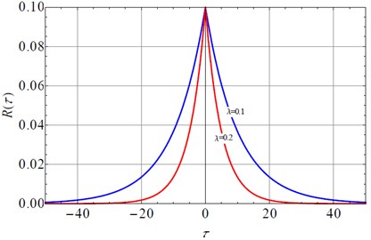
However, we must pay attention to the importance of the colored noise excitations. As is well known, Gaussian colored noise, which can be obtained by a zero-mean Gaussian white noise passing through a linear filter $\dot{\eta }=-\lambda \eta +\lambda \xi \left(t\right)$, is a better approximation of the natural ambient noise than the white noise, and has the correlation function in the form of:

where $\lambda$ denotes the correlation time parameter and $\xi \left(t\right)$ denotes a Gaussian white noise with 0 mean and intensity of 2$D$. The expression of Eq. (1) can be also seen in reference [28]. If $D=$1, $\lambda =\mathrm{}$0.1, 0.2, Fig. 1 shows the diagram of the correlation function $R.$ As is well known, the autocorrelation function of the white noise is $R\left(\tau \right)=\mathrm{E}\left[\xi \right(t\left)\xi \right(t+\tau \left)\right]=D\delta \left(\tau \right)$, the $\delta \left(\tau \right)$ is the Dirac delta function. If the parameter $\lambda$ in Eq. (1) is infinitely large, the colored noise will decrease to be a Gaussian with noise. G. Falsone and I. Elishakoff [29] developed a stochastic linearization technique for colored noise excited Duffing oscillator. After that, Bo Li et.al. [30] and Gen Ge. et al. [31] extended the stochastic averaging method into wider fields such as nonlinear oscillator with stiffness nonlinearity and inertia nonlinearity.

The detailed response characters of colored noise excited piezoelectric cantilever model, such as stationary probability density function (PDF) of displacement, PDF of voltage, joint PDF of displacement and velocity and mean square values of voltage, haven’t been studied yet. Thus, a method on stationary responses of piezoelectric cantilever with colored noise excitation is proposed in this paper.

The research subject is a uniform cantilever with two layers of piezoelectric ceramic on the top as well as the bottom. The linear strain-stress relation as well as the nonlinear deformation is taken into account. Firstly, the dynamic model is built by the Lagrange equation and is transformed into dimensionless form. Secondly, a pair of differential equations of amplitude and phase is obtained by coordinate transformation. After that, the pair of equations is simplified to be an Itô type stochastic differential equation. Thirdly, the stationary probability density functions about the amplitude, the displacement and the output voltage, the joint probability density function of the displacement and velocity, as well as the mean square value of voltage, are all obtained by solving the averaged Fokker-Plank-Kolmogorov (FPK) equation. At last, the influence of the noise density and the noise delay time on these PDFs are also studied. The Monte Carlo simulations verifies this procedure.

Fig. 1The correlation function of the colored noise

2. The modeling

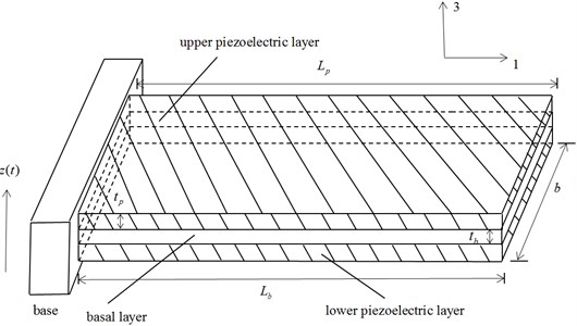
As is shown in Fig. 2, the piezoelectric cantilever is characterized as: the thickness of the piezoelectric ceramic $t_p$, the length of the base beam $L_b$, the width of the cantilever. The vector 1 denotes the longitudinal direction, while vector 3 denotes the transversal direction. $z\left(t\right)$ is the pedestal excitation in the form of colored noise.

Fig. 2Cantilever beam with piezoelectric sheets fully covered under excitation of base noise

The strain-stress relation of the piezoelectric ceramic is expressed as [1]:

where, $T_1^p$ denotes the 1-direction stress of ceramic, $S_1^p$denotes the 1-direction strain of ceramic, $C_{11}^E$denotes Young’s modulus of elasticity of piezoelectric ceramic, $E_3$ denotes 3-direction electric field intensity, $D_3$ denotes 3-direction potential shift.

Although every mode can be excited by the colored noise, the first mode’s amplitude predominates those of the lower modes. Thus, only the first mode is studied. It is assumed that the point away from the base has the transverse displacement $w\left(s,t\right)=\phi \left(s\right)q\left(t\right)$, where $\phi \left(s\right)$ is the first order mode function, and $q\left(t\right)$ denotes the modal coordinate. The piezoelectric cantilever stores up the kinetic energy, the elastic potential energy and the electric energy. The kinetic energy of the base layer and that of one piece of piezoelectric ceramic are as follows:

In Eq. (4) and Eq. (5), ${\rho }_b$ denotes the density of the base layer, ${\rho }_p$ denotes the density of the ceramic, $\dot{w}+\dot{z}$ denotes the transverse velocity.

The strain of the point away from the neutral layer with distance y is expressed as: $S_1^p=-yw\text{'}\text{'}$.

The total elastic energy is:

where $v_p$ denotes the volume of the piezoelectric ceramic, $I_p=b{\int }_{\frac{t_b}{2}}^{\frac{t_b}{2}+t_p}{y}^{2}dy$ is the inertia moment to the neutral layer, ${I_p}^{\text{'}}=b{\int }_{\frac{t_b}{2}}^{\frac{t_b}{2}+t_p}{y}^{4}dy$ is the fourth-order moment to the neutral layer, $d=\frac{t_b+t_p}{2}$ denotes the distance from the center of the ceramic layer to the neutral layer. Thus, one has:

The work done by the electric force is:

The Lagrange function is defined as $L=T-U+W_e$. Considering the damping dissipation energy $\psi ={\int }_0^L\frac{1}{2}C{\dot{w}}^{2}ds$, the Lagrange equation is written as follows:

Integrating $D_3$ on the ceramic surface aero, the electric quantity $Q\left(t\right)$ passing through $R_L$ is:

Taking derivative to $Q\left(t\right)$ with respect to time $t$, and considering the Ohm law, the electric current $I\left(t\right)$ satisfies:

where, the electric capacity is $C_p=\frac{{{\epsilon }_{33}}^{S}b{L}_p}{2t_p}$.

The piezoelectric function is:

Introducing the character length and the character time scale, the dimensionless transformation is as follows:

The dynamic equation and the piezoelectric equation are obtained as:

where parameters are:

By defining $\mu =\frac{c^{\mathrm{*}}}{h_1}$, ${{\omega }_0}^2=\frac{h_2}{h_1}$, $\alpha =\frac{h_3}{h_1}$, $\vartheta =\frac{h_4}{h_1}$, $\eta =\frac{h_5}{h_1}\ddot{f}$, Eq. (13) and Eq. (14) can be transformed as:

Parameters in Eq. (15) and Eq. (16) are as follows: ${\omega }_0$ denotes the fundamental frequency, $\alpha$ is the cubic nonlinearity coefficient, $\mu$ is the damping ratio, $\beta$ and $\vartheta$ are electromechanical coupling coefficient in piezoelectric equation and that in dynamic equation, $\eta \left(t\right)$ denotes the colored noise.

3. Stochastic averaging

Standard stochastic averaging method is an effective tool in dealing with quasi-linear oscillators subject to wide band noise. When the nonlinear stiffness term is weak enough, it has weak influence on the responsive frequency. The model we use in this paper has weak nonlinearity when the deformation is small.

For convenience, the dimensionless time $\tau$ is still expressed as $t$:

where $\theta ={\omega }_{0}t+\phi$.

Substituting Eq. (17) into Eq. (16), one has:

Then the voltage can be expressed as:

where $B=\sqrt{{B_1}^2+{B_2}^2}=\frac{A\beta {\omega }_0}{\sqrt{{\gamma }^2+{{\omega }_0}^2}}$, ${\phi }_u=\phi +\mathrm{\Delta }\phi$, $\mathrm{t}\mathrm{a}\mathrm{n}\phi =\frac{B_1}{B_2}=-\frac{\gamma }{{\omega }_0}$.

The presumption of the transformation is that the nonlinear term has weak influence on the frequency. Subsequently the responsive frequency is still assumed to be ${\omega }_0$. The correctness of this assumption will be verified in the numerical simulation section.

Taking derivative to $x=A\mathrm{c}\mathrm{o}\mathrm{s}\theta$, $y=-A{\omega }_0\mathrm{s}\mathrm{i}\mathrm{n}\theta$ with respect to time $t$ yields:

Solving the two equations, one can obtain:

By now, a pair of stochastic differential equation has been solved out which can be expressed in the standard form:

where:

An Itô type stochastic differential equation of the limiting diffusion process can be given as:

where $m\left(A\right)$ denotes the drift coefficient, ${\sigma }^2\left(A\right)$ denotes the diffusion coefficient, $W\left(t\right)$ is standard unit Brownian motion (see reference [29, 30]). The operator $⟨•⟩=\frac{1}{2\pi }{\int }_0^{2\pi }•d\theta$ does averaging with respect to time, $R\left(\tau \right)$ denotes the noise correlation function, 2D is the noise strength, $\lambda$ is the time delay coefficient:

where $E⟨•⟩$ denotes the mathematical expectation, $\delta \left(\tau \right)$ is the Dirac-delta function.

For application, people pay more attention to the amplitude than to the phase. Using the Eq. (26), the drift coefficient $m\left(A\right)$, and the diffusion coefficient ${\sigma }^2\left(A\right)$ are given as:

Thus the Eq. (22) can be averaged to be Eq. (30):

4. Stationary responses

The averaged Fokker-Plank-Kolmogorov (FPK) equation associated with Itô equation (30) is of the form:

where $p(A,t)$ is the transition probability density of displacement amplitude $A$. Under assumption that zero probability flows at the two boundaries $A=0$ and $A=\mathrm{\infty }$, the stationary solution of FPK equation $p\left(A\right)$ for Eq. (31) is of the form:

where constant $N$ is the normalization constant.

Substituting Eq. (28), Eq. (29) into Eq. (32) yields the stationary PDF of the equivalent amplitude:

Considering the relation $B=\frac{A\beta {\omega }_0}{\sqrt{{\gamma }^2+{{\omega }_0}^2}}$ one can deduce the PDF of the output voltage as:

The joint stationary probability density of displacement$x$and velocity $y=\dot{x}$ can be further obtained from $p\left(A\right)$ as follows:

Subsequently, the PDF of displacement $p\left(x\right)$ can be gained by integrating $y$ form –∞ to ∞ in Eq. (35):

On the other hand, by integrating $x$ form –∞ to ∞ in Eq. (35), the PDF of velocity $p\left(y\right)$ can also be obtained.

Considering the relation $p\left(u\right)={\left.\frac{1}{2\pi \omega B}p\left(B\right)\right|}_{B\to \sqrt{u^2}}$, PDF of the output voltage $p\left(u\right)$ is:

By Eq. (18), one knows $u=-\frac{\beta {{\omega }_0}^2}{{\gamma }^2+{{\omega }_0}^2}x-\frac{\beta \gamma }{{\gamma }^2+{{\omega }_0}^2}y$, thus the mean square value of voltage is:

From Eq. (33) to Eq. (38), one has obtained all theoretical predictions in need to investigate the efficiency of collecting the electric energy. In the nest section, necessary numerical simulations will be carried out to verify these equations.

5. Numerical simulation

The Monte Carlo method is applied to verify the effectiveness of the above Eq. (33), Eq. (35), Eq. (35), Eq. (37) and Eq. (38). The parameters are set as: ${\omega }_0=$ 1, $\mu =$0.05, $\alpha =$ 1, $\beta =$ 0.01, $\gamma =$0.1, $\vartheta =$ 0.05. The parameter D is chosen as $D=$0.001 and $D=$0.002, separately. As is well known, the larger the correlation time parameter is, the narrower the noise band becomes. The time delay coefficient is chosen as $\lambda =$0.5 and $\lambda =$5 for comparison. Totally 3,000 sets of colored noise are imposed to the Eq. (15) and Eq. (16). Each set of noise includes 30,000 numbers. The time step is set as $\mathrm{\Delta }t=\text{0.005}$. The numerical solutions could be obtained by an order-2 stochastic Runge-Kutta algorithm [31]. The last 10,000 steps are kept as the stationary responses. For each step the transient amplitude $A=x^2+\frac{y^2}{{{\omega }_0}^2}$ is calculated out. Finally, do statistic on total stationary $n=$3,000×10,000 values of $A$, $x$, and $u$, and the stationary probability density functions of the amplitude $p\left(A\right)$, of the displacement $p\left(x\right)$, of the voltage $p\left(u\right)$ are shown in Fig. 3-Fig. 5.

Fig. 3The analytical solution and numerical solution of stationary PDF of amplitude (solid lines: Eq. (33) dots: Monte Carlo simulation on Eq. (15) and Eq. (16))

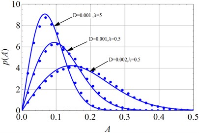
Fig. 4The analytical solution and numerical solution of stationary PDF of displacement (solid lines: Eq. (36); dots: Monte Carlo simulation on Eq. (15) and Eq. (16))

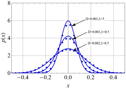
From Fig. 3-Fig. 5, one can easily find that larger noise density will induce wider spread of the amplitude, displacement and voltage. And, with the same noise density, smaller time delay coefficient $\lambda$ i.e. wider noise band, will clearly lead to wider spread of these three variables. Also, it is obvious that the numerical simulation coincides with the theoretical prediction.

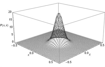
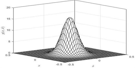
Subsequently, the joint PDF of displacement $x$ and velocity $y=\dot{x}$ are numerically simulated. We take 40×40 grids in a range $\left\{-0.5\le x\le 0.5,-0.5\le y\le 0.5\right\}$ with a space gap: $\mathrm{\Delta }x=\mathrm{\Delta }y=\text{0.025}$. Then we count the numbers $n_{ij}$ ($i$, $j=$1-40) of the $n=$4,000×10,000 stationary $\left(x,y\right)$ dots which fall within each grid. Finally, the joint PDF $p\left(x,y\right)$ value of each grid can be calculated out by $p\left(x_i,y_i\right)=\frac{n_{ij}}{n\times \mathrm{\Delta }x\times \mathrm{\Delta }y}$. The joint PDF are illustrated in Fig. 6.

Fig. 5The analytical solution and numerical solution of stationary PDF of voltage (solid lines: Eq. (37); dots: Monte Carlo simulation on Eq. (15) and Eq. (16))

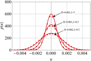
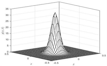
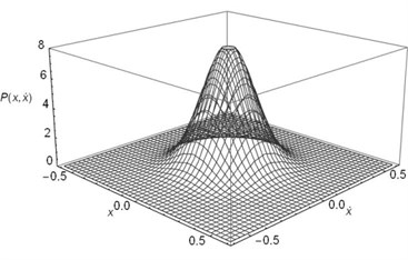
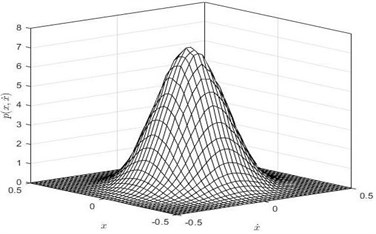
Fig. 6The joint stationary PDF of displacement x and velocity y: a), b) for D= 0.001, λ = 0.5, c), d) for D= 0.001, λ = 5; e, f) for D= 0.002, λ = 0.5; a), c), e) are given by Eq. (35); b), d), f) are obtained by Monte Carlo simulation)

a)

b)

c)

d)

e)

f)

Obviously, Fig. 6 gives a full view of the probability density function of the displacement and velocity. If one do integral to PDF $p\left(x,y\right)$ with respect to variable y from $-\mathrm{\infty }$ to $+\mathrm{\infty }$, the joint PDF will degrade to the PDF of displacement $p\left(x\right)$ as shown in Fig. 4. Similarly, the larger the noise density $D$ is and the smaller the time delay coefficient is, the lower peak value of the Fig. 6 becomes.

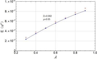
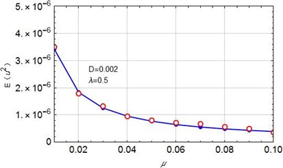
Fig. 7Mean square values of voltage with different coefficients: a) for D= 0.002, μ= 0.05; b) for D= 0.002, λ= 0.5; The solid line is the theoretical prediction value obtained by Eq. (38), and the hollow circle is the numerical result obtained by Monte Carlo simulation)

a)

b)

Mean square value of the output voltage $E\left(u^2\right)$ is an important index in estimating the piezoelectric cantilever’s behavior. One can see the output $E\left(u^2\right)$ is basically proportional to the time delay factor $\lambda$ from 0.3 to 0.9. As is well known, the larger the time delay factor $\lambda$ is, the wider the noise band becomes. There comes the conclusion that the wider band noise will lead to larger voltage output even if the noise has the same noise density. Also, it is not hard to understand that when the damping increases the output will decrease in Fig. 7(b). This finding is consistent with the conclusion given by Daqaq [23].

6. Conclusions

A piezoelectric cantilever model subject to colored noise is studied and the stationary responses are theoretically predicted by applying the stochastic averaging method. Generally, this is an effective method which enriches the methods in random vibrational field of the piezoelectric cantilever. Some conclusions are summarized as follows:

1) The Cubic nonlinear coefficient $\alpha$ has small influence on the responses. In the theoretical prediction equations of amplitude, displacement, voltage, (see Eq. (34-39)), the coefficient $\alpha$ was eliminated during the stochastic averaging procedure. But the good fitness between the equations and the numerical simulation shows this coefficient $\alpha$ has few impacts on these responses. This phenomenon coincides with the reference [24].

2) Stronger noise intensity will not only lead to larger vibration amplitude and displacement but also lead to lager output mean square voltage. Time delay factor also has a significant influence on the output mean square voltage. With the same noise density level, the larger the time delay factor is (i.e. the wider the noise band is), the larger the voltage output becomes.