Abstract
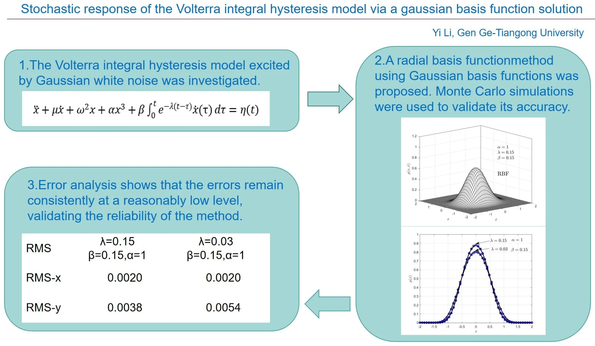
This paper investigates the random response of hysteretic nonlinear oscillators described by the Volterra integral model, which captures material memory effects via a convolution kernel under Gaussian white noise excitation. The Gaussian basis function (GBF) approximation technique is utilized to estimate the system's steady-state probability density function (PDF). The approximately stationary probability density function is represented as a weighted sum of Gaussian basis functions in this method. The optimal weighting coefficients are determined by minimizing the residual of the stationary Fokker-Planck-Kolmogorov (FPK) equation using the least squares method with Lagrange multipliers, yielding the steady-state joint probability density function. The computed results show excellent agreement with Monte Carlo simulations (MCS), confirming the accuracy and reliability of the Gaussian basis function method and demonstrating the influences of various parameters on the hysteresis loop and the system response.
Highlights
- The Gaussian basis function (GBF) method is applied to solve the steady-state response of a Volterra integral hysteretic system under Gaussian white noise excitation.
- The non-monotonic effect of the Volterra kernel decay rate on the hysteresis loop area and the steady-state probability density function is revealed.
- The memory damping strength coefficient and the nonlinear stiffness coefficient have a significant influence on the peak value of the probability density function.
- Error analysis shows that the root-mean-square error remains at a reasonably low level under different parameters, verifying the reliability and applicability of the GBF method for strongly memory-dependent hysteretic systems.
1. Introduction
Hysteretic nonlinear systems have broad applications in various engineering domains, including viscoelastic composite dampers [1] and other related fields [2-3]. For example, Humaidi et al. developed various advanced nonlinear control schemes for magnetorheological dampers (MRDs) in the seismic vibration control of buildings [4-6]. The common feature of hysteretic nonlinear systems is that their mechanical response depends not only on the current input but also on the past loading history, which results in a memory effect.
Several models have been developed for hysteretic nonlinear systems, including the Bouc-Wen model [7], the bilinear model [8], the Duhem model [9], the Preisach model [10], among others. The Volterra integral model represents one such approach and stands out because of its clear physical basis and flexible parameter tunability. It employs a convolution integral with an exponentially decaying kernel, expressing the current stress as the sum of an instantaneous nonlinear strain term and a weighted cumulative term that accounts for the history of strain rates, thereby naturally capturing the material's memory. Its integral-type constitutive relation is physically transparent, and by adjusting the memory kernel, various hysteresis loop shapes can be reproduced. Furthermore, unlike several conventional models, the model is characterized by a relatively concise set of parameters, and its formulation does not require piecewise functions.
When such systems are subjected to random environmental excitations, their responses become stochastic and must be treated within a probabilistic framework. The evolution of the response probability density function is governed by the Fokker-Planck-Kolmogorov (FPK) equation. For the Volterra integral model with an exponentially decaying kernel, the FPK equation is a standard partial differential equation, and the Volterra integral model has the advantage of being transformable into a standard three-dimensional Markov system. However, even this FPK equation remains difficult to solve analytically. Traditional approximate methods (such as equivalent linearization [11]-[13], the moment method [14], and the stochastic averaging method [15]-[17]) often introduce significant errors when dealing with such strongly memory-dependent systems because they either ignore the cumulative historical effects or oversimplify the kernel function structure. This limitation is particularly severe when the kernel decay rate is moderate or small, severely restricting the applicability of these methods.
In recent years, semi-analytical methods based on the least-squares fitting approach with radial basis functions have shown great potential in stochastic dynamics [18] and other related fields [19]-[25]. These methods represent the unknown probability density function as a weighted sum of Gaussian basis functions and determine the weight coefficients by minimizing the residual sum of squares of the FPK equation at sample points, thereby transforming the solution of the partial differential equation into an algebraic optimization problem. This approach exhibits good robustness to the type and strength of system nonlinearity. It has been successfully applied to the stochastic response analysis of various hysteretic and strongly nonlinear systems. Chen et al. used this method to analyze the response of Duhem models under harmonic and random excitations [26], as well as the stochastic response of Bouc-Wen systems when excited by Poisson white noise [27].
In this paper, we investigate the steady-state stochastic response of a hysteretic system described by the Volterra integral model under Gaussian white noise excitation. First, we establish the differential equation of motion of the system and analyze the influence of the memory kernel parameters on the area and morphology of the hysteresis loop. Then, based on the Gaussian basis function (GBF) fitting method, we derive semi-analytical expressions for the stationary joint probability density function and the marginal PDFs of the system. Finally, a comparison with MCS is performed. This study aims to 1) reveal the non-monotonic regulatory mechanisms of key parameters – such as the memory kernel decay rate, the memory damping strength, and the nonlinear stiffness – on the response probability distribution and to uncover the physical mechanism of “memory-induced stiffness” induced by the cumulative effect of historical strain rates when the kernel decay rate is extremely small; 2) verify the computational accuracy and applicability of the GBF method for the Volterra integral hysteresis model; and 3) provide methodological support for the stochastic vibration analysis and parameter optimization of hysteretic models with strong memory effects.
2. Model
2.1. Volterra integral model
This paper introduces a theoretical stress–strain model with hysteretic characteristics. The governing equation is shown in Eq. (1):
where represents stress, represents strain, is the linear elastic modulus, represents the nonlinear elastic modulus, represents the Volterra integral. is the Volterra integral memory kernel function, represents the decay rate of the Volterra kernel function, is the current time, and represents a past moment. The integral indicates the weighted influence of the strain rate at past moments on the current stress. The images of the stress-strain model are shown in Fig. 1.
In Fig. 1(b), the stress-strain relationship diagram exhibits a hysteresis loop, which can be interpreted as the current stress always being related to the strain over a past period.
Fig. 1Volterra integral of the stress-strain model
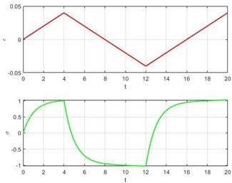
a) Strain-time and Stress-time curve
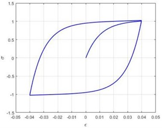
b) Stress-strain relationship curve (schematic)
2.2. Parameter influence on the Volterra integral
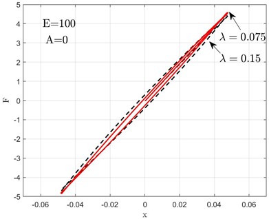
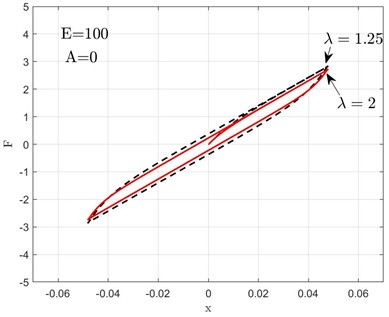
With the Volterra kernel function decay rate 0.15 and the linear elastic modulus taken as 100 and 75, the Volterra integral hysteresis loops are plotted in Fig. 2. When the linear elastic modulus is taken as 100 and the Volterra kernel function decay rate is taken as 0.15 and 0.075, the Volterra integral hysteresis loops are presented in Fig. 3(a); when is taken as 1.25 and 2, the hysteresis loops are presented in Fig. 3(b); when is taken as 0 and 7e3, the hysteresis loops are presented in Fig. 4.
Fig. 2Volterra integral hysteresis loops under different linear elastic moduli
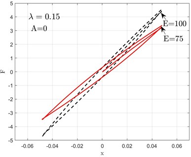
Fig. 3Volterra integral hysteresis loops under different Volterra kernel function decay rates
a)
b)
Fig. 4Volterra integral hysteresis loops under different nonlinear elastic moduli
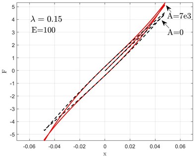
Figs. 2-4 show that when the linear elastic modulus decreases, the hysteresis loop undergoes a marked change in shape, the material stiffness decreases, and the overall vertical position of the loop decreases (because the elastic part diminishes), but the hysteresis loop exhibits no change in width. That is, when decreases, the hysteresis loop exhibits a constant area, and the loop shifts downward overall in the stress direction, resulting in a flatter profile, but the dissipated energy remains unchanged. When is very small, as the Volterra kernel function decay rate increases, the hysteresis loop substantially increases in area. However, as continues to increase, the hysteresis loop area decreases instead. As the nonlinear elastic modulus increases, the area of the hysteresis loop remains unchanged, but its shape transforms into an “S” shape. It is evident that the linear elastic modulus and the nonlinear elastic modulus are key factors determining the shape of the Volterra integral hysteresis loop. The area of the Volterra integral hysteresis loop is determined by the Volterra kernel function decay rate , and it also depends on loading characteristics.
2.3. Model and its FPK equation
The dynamic model developed in this paper represents a single-degree-of-freedom hysteretic system with a Volterra integral constitutive relation. Its hysteretic behavior follows the Volterra integral constitutive law detailed in Section 2.1. The dimensionless equation of motion for this system is given by Eq. (2):
where is time; is displacement; is velocity; is acceleration; is the strength coefficient of the memory damping term, determining the influence degree of the past velocity history on the current system dynamics; represents Gaussian white noise excitation. Here, is the Volterra integral function denoted by , as shown in Eq. (3):
where represents the Volterra kernel function decay rate, a parameter measuring the decay rate of the material's memory effect over time. Within a certain range, a larger value indicates that the influence of past strain on the current stress decays faster, and the material's historical dependence is weaker. When it is sufficiently small, the system retains memory of strain histories over multiple loading cycles, resulting in a more complex hysteretic response. represents Gaussian white noise with intensity , i.e., , where refers to the standard Wiener process.
Let , Eq. (2) can be written in Itô equation form:
The Itô stochastic differential equation takes the following standard form:
where represents the drift term and represents the diffusion term.
According to Eq. (4-5), we obtain:
Eq. (5) is written as the standard FPK equation:
The FPK equation for Eq. (4) is:
By setting 0, the system’s steady-state PDF satisfies:
The condition 0 means that over a sufficiently long time, the probability function remains unchanged. Our objective is to derive a high-accuracy approximate PDF for this steady-state solution.
3. Methodology
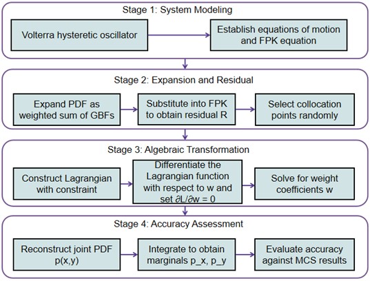
We employ the RBF method [28], where the output is formed by summing Gaussian basis functions each multiplied by its corresponding weight coefficient. This sum is used to represent the steady-state solution of Eq. (9), denoted as :
where the subscript denotes the -th Gaussian basis function. represents the weight coefficient, denotes the standard deviation, denotes a Gaussian basis function:
where , , is the Euclidean norm, representing the distance between the input coordinate and the center point coordinate . We select a domain in the space, then divide it into 18×18×18 grid points, with each grid point serving as a GBF center, i.e., = . represents the variance, and the smaller it is, the sharper the function graph becomes. Setting the basis function variance to yields a moderate shape, where denotes the maximum distance between any two center points. This choice ensures sufficient overlap between adjacent basis functions, thereby avoiding numerical ill-conditioning.
Fig. 5Flowchart of the proposed solution procedure
Define a function as the residual between and :
Plugging Eq. (10) into Eq. (12), the residual can be rewritten as:
where denotes the error function.
The following normalization condition holds for all between and the GBF:
The conditions on the weight coefficients are:
We define a sampling domain . Here denotes the total number of sampling points. Typically, is between and 2.5 to ensure that the sampling points completely cover the effective support regions of all basis functions. This is a common practice to guarantee a well-conditioned interpolation matrix, so . We set = . The sampling density is far higher than the theoretical threshold required to ensure convergence of the discrete approximation to the continuous solution, which guarantees the accuracy of the approximation. The Lagrangian function is then constructed based on the FPK residual evaluated at randomly sampled collocation points:
The necessary condition for minimizing is:
They are expanded into matrix form as:
where the error matrix is expressed as:
The optimal weight coefficient is represented in vector form:
Substituting the into the error function in Eq. (21) and calculating the vector in Eq. (22), we obtain the weight coefficients.
We acquire the approximate PDF . Then, integrating yields the marginal PDF:
Here, we adopt the root mean square error (RMS) of the PDF solution as the metric to quantify the error of the Gaussian basis function fitting:
where is the PDF value from MCS (a 4th-order stochastic Runge-Kutta algorithm [29]) at point ; is the corresponding value from the RBF method. For Eq. (2), 3000 independent noise realizations are generated. Each noise sequence contains 10,000 points, with the last 6,000 points of the response considered the steady-state response. Then, the simulation time step is 0.04. The final 3,000×6,000 simulated points serve to statistically determine the probability of each grid falling within the - plane. The following sections present comparisons between the GBF and MCS results. The computed results are listed in Table 1.
4. Numerical simulation and error analysis
4.1. Effect of the Volterra kernel decay rate
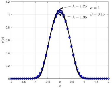
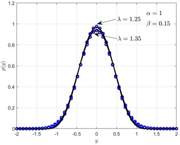
With parameters fixed at = 1, = 0.15, is taken as 1.25 and 1.35 to examine how influences the system when it takes large values.
From Fig. 7, when the decay rate of the Volterra memory kernel is relatively large, a further increase in leads to consistent variations between the PDF profiles and the hysteresis loops. The underlying physical mechanism is that excessively rapid decay of the kernel restricts significant contributions to the current stress solely to strain rates at very recent past instants. Consequently, the equivalent damping supplied by the memory damping term diminishes, reducing the system’s overall energy dissipation capacity, which in turn amplifies the amplitudes of both the displacement and velocity responses. On the steady-state probability density function, this behavior manifests as a lowered peak and broadened tails. Thus, it can be concluded that in this case, the Volterra kernel function decay rate is negatively correlated with the hysteresis loop area.
Fig. 6Joint probability density plots for different values of the Volterra kernel function decay rate
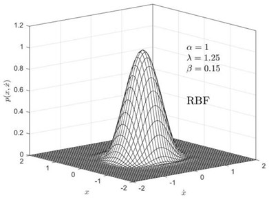
a) = 1.25 RBFNN outcomes
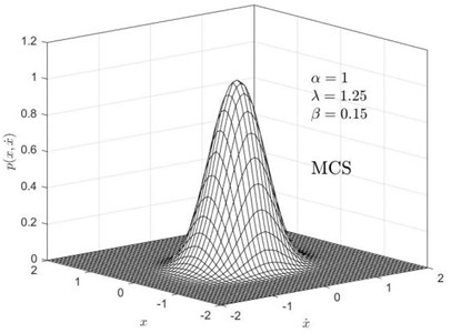
b) = 1.25 Monte Carlo simulation
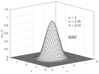
c) = 1.35 RBFNN outcomes
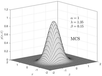
d) = 1.35 Monte Carlo simulation
Fig. 7Influence of the Volterra kernel function decay rate on the displacement and velocity probability densities: a) shows px, b) shows py. Solid lines represent RBF, circles represent MCS
a)
b)
Parameters are fixed at = 1, = 0.15, with taken as 0.15 and 0.03 to examine how the decay rate of the Volterra kernel function influences the system when is small.
From Fig. 9, it can be seen that when is very small, the system has a long memory time, and the stress is influenced by the deformation history from much earlier times, potentially retaining “memory” of strain rates from multiple past cycles. This leads to stress responses that are not only related to current strain but also to multiple historical cycles. The hysteresis loop becomes wider or exhibits complex time-delayed responses, and the energy dissipation characteristics vary more gradually with frequency. That is, a smaller leads to lower peaks and a wider distribution range in the displacement and velocity probability density images. For an extremely small of the Volterra memory kernel, the memory term ceases to function solely as a damping element and approximates a history-dependent elastic constraint. Thus, it can be concluded that in this case, the Volterra kernel function decay rate is positively correlated with the hysteresis loop area.
The decay rate of the Volterra memory kernel governs the fading rate of the material’s memory of past strain rates, and it exerts an inherently non-monotonic influence on both the hysteresis loop area and the system’s steady-state response. For a single exponential kernel, this non-monotonic behavior is related to its frequency-dependent equivalent stiffness and damping. This non-monotonic effect, by modifying the probability density function shape, can provide a basis for parameter design in structural vibration control and also serve as an indicator for assessing material aging conditions.
Fig. 8Joint probability density plots for different values of the Volterra kernel function decay rate
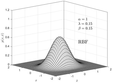
a) = 0.15 RBFNN outcomes
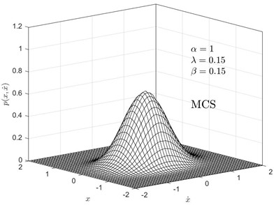
b) = 0.15 Monte Carlo simulation
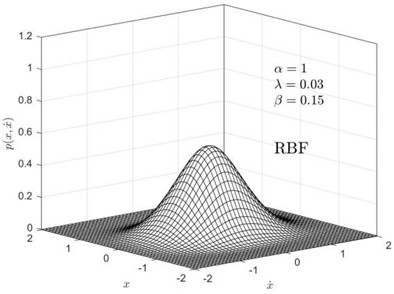
c) = 0.03 RBFNN outcomes
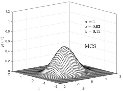
d) = 0.03 Monte Carlo simulation
Fig. 9Influence of the Volterra kernel function decay rate on the displacement and velocity probability densities: a) shows px, b) shows py. Solid lines represent RBF, circles represent MCS
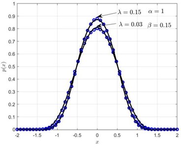
a)
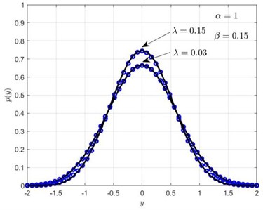
b)
4.2. Effect of memory damping strength coefficient
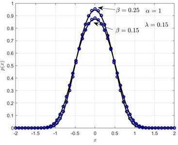
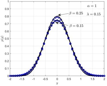
Parameters are fixed at = 0.15, = 1, with taken as 0.15 and 0.25 to examine how the memory damping strength coefficient influences the system.
From Figs. 10-11, with increasing memory damping strength coefficient , the peaks of the displacement and velocity PDFs increase, whereas the bell-shaped distribution ranges become narrower. Thus, it can be concluded that a larger memory damping strength coefficient results in higher peaks.
Fig. 10Steady-state probability density plots for two different memory damping strength coefficient values
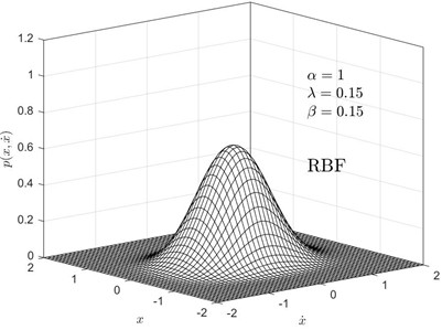
a)= 0.15 RBF outcomes
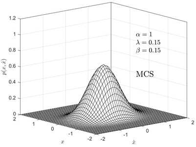
b)= 0.15 Monte Carlo simulation
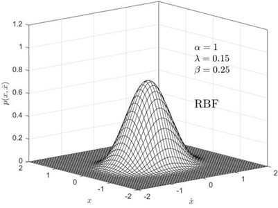
c) = 0.25 RBF outcomes
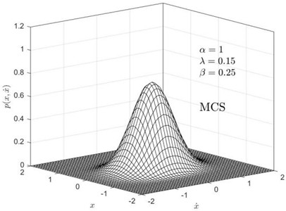
d)= 0.25 Monte Carlo simulation
Fig. 11Probability density of displacement and velocity for two different memory damping strength coefficient values: a) shows px, b) shows py. Solid lines represent RBF, circles represent MCS
a)
b)
4.3. Effect of the nonlinear stiffness coefficient
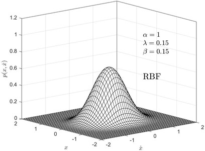
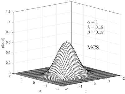
Parameters are fixed at = 0.15 and = 0.15, with taken as 1 and 1.8 to examine the effect of the nonlinear stiffness coefficient on the steady-state response.
The nonlinear stiffness coefficient is the dimensionless form of the cubic nonlinear coefficient defined in Section 2.1. It changes the stiffness distribution of the system, without altering the dissipative characteristics of the Volterra hysteresis term, but it significantly affects the probabilistic distribution characteristics of the response. Fig. 13 shows that as the nonlinear stiffness coefficient increases, the peaks of the curves increase significantly, and the coverage range of the curves becomes narrower. Thus, it can be concluded that a larger nonlinear stiffness coefficient results in higher peaks and has a relatively large influence on the steady-state PDF of displacement and velocity.
Fig. 12Joint probability density plots for different values of the nonlinear stiffness coefficient
a)= 1 RBF outcome
b)= 1 Monte Carlo simulation
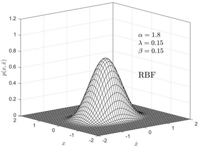
c)= 1.8 RBF outcomes
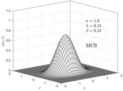
d)= 1.8 Monte Carlo simulation
Fig. 13Probability densities p(x) and py for different values of the nonlinear stiffness: a) shows px, b) shows py. Solid lines represent RBF, circles represent MCS
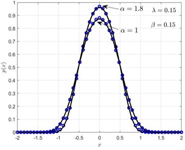
a)
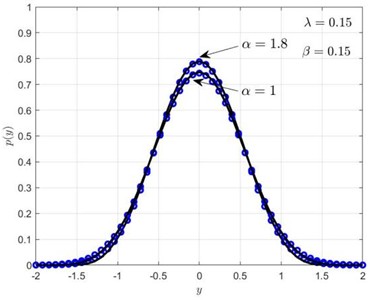
b)
4.4. Error analysis
The root mean square errors obtained by the two methods under different parameter conditions are calculated and listed in Table 1, indicating that the errors consistently remain at a reasonably low level. These numerical results strongly support that the RBF method possesses high computational accuracy and reliability.
Table 1Root mean square error under different parameters
RMS | = 1.25 = 0.15, = 1 | = 1.35 = 0.15, = 1 | = 0.15 = 0.15, = 1 |
RMS- | 0.0099 | 0.0073 | 0.0020 |
RMS- | 0.0105 | 0.0121 | 0.0038 |
RMS | = 0.03 = 0.15, = 1 | = 0.15 = 0.25, = 1 | = 0.15 = 0.15, = 1.8 |
RMS- | 0.0020 | 0.0064 | 0.0046 |
RMS- | 0.0054 | 0.0093 | 0.0066 |
5. Conclusions
Addressing the response problem of hysteretic nonlinear systems under random excitation, this paper describes their constitutive relationship based on the Volterra integral model. The GBF fitting method is extended to this case. The summary is as follows:
1) In Table 1, the proposed GBF approach demonstrates reliability in analyzing Volterra integral hysteretic nonlinear oscillators.
2) The physical meaning of the hysteresis loop parameters in the Volterra integral model is clear. The decay rate plays a key role in determining the hysteresis loop area. Changes in the linear elastic modulus do not alter the dissipated energy, leaving the hysteresis loop area constant, but the loop shifts overall in the stress direction; the nonlinear elastic modulus does not change the area of the hysteresis loop, but it does change its shape.
3) The decay rate of the Volterra kernel exerts a non-monotonic regulatory effect on the system response. When is relatively large, the material exhibits short memory retention, causing the hysteresis loop to contract, so the peak value of the PDF decreases. Conversely, when is small, long-term memory effects become significant: the accumulation of historical strain rates effectively enhances the system’s equivalent stiffness, which suppresses the response amplitude and leads to an increase in the PDF peak. This phenomenon is referred to as the “memory-induced stiffness” effect.
4) represents the cubic nonlinear term in the constitutive equation, and is its dimensionless nonlinear stiffness coefficient. They do not alter the dissipative characteristics of the system. However, it does change the stiffness distribution of the system, thereby significantly affecting the probabilistic characteristics of the response. As the nonlinear stiffness coefficient increases, the peak becomes higher, and the distribution range becomes narrower. As increases from 1 to 1.8, increases from 0.87 to 0.96, and increases from 0.74 to 0.78. When increases from 0.15 to 0.25, increases from 0.87 to 0.94, and increases from 0.74 to 0.8.
Future work will extend the proposed method to the dynamic analysis of nonlinear mechatronic systems with hysteresis and uncertainties [30].
References
-
H. Zhang, A. Li, Y. Su, G. Xu, and B. Sha, “Viscoelastic dampers for civil engineering structures: a systematic review of constructions, materials, and applications,” Journal of Building Engineering, Vol. 96, p. 110597, 2024, https://doi.org/10.1016/j.jobe.2024.110597
-
S. Yang and Y. Shen, “Recent advances in dynamics and control of hysteretic nonlinear systems,” Chaos, Solitons and Fractals, Vol. 40, No. 4, pp. 1808–1822, 2007, https://doi.org/10.1016/j.chaos.2007.09.064
-
J. Cai, W. Dong, and R. Nagamune, “A survey of Bouc-Wen hysteretic models applied to piezo-actuated mechanical systems: modeling, identification, and control,” Journal of Intelligent Material Systems and Structures, Vol. 34, No. 16, pp. 1843–1863, 2023, https://doi.org/10.1177/1045389x231157361
-
A. J. Humaidi, M. E. Sadiq, A. I. Abdulkareem, I. K. Ibraheem, and A. T. Azar, “Adaptive backstepping sliding mode control design for vibration suppression of earth-quaked building supported by magneto-rheological damper,” Journal of Low Frequency Noise, Vibration and Active Control, Vol. 41, No. 2, pp. 768–783, 2021, https://doi.org/10.1177/14613484211064659
-
A. Q. Al-Dujaili, A. J. Humaidi, Z. T. Allawi, and M. E. Sadiq, “Earthquake hazard mitigation for uncertain building systems based on adaptive synergetic control,” Applied System Innovation, Vol. 6, No. 2, p. 34, 2023, https://doi.org/10.3390/asi6020034
-
N. Q. Yousif, S. S. Husain, O. H. Abdullah, A. J. Humaidi, and A. K. Al-Mhdawi, “RISE control design to reduce earthquake effect on building structures with MRD,” J. Eng. Sci. Technol, Vol. 20, No. 5, pp. 1568–1581, 2025.
-
Y.-K. Wen, “Method for random vibration of hysteretic systems,” Journal of the Engineering Mechanics Division, Vol. 102, No. 2, pp. 249–263, 2021, https://doi.org/10.1061/jmcea3.0002106
-
T. K. Caughey, “Random excitation of a system with bilinear hysteresis,” Journal of Applied Mechanics, Vol. 27, No. 4, pp. 649–652, 1960, https://doi.org/10.1115/1.3644077
-
A. Visintin, Applied Mathematical Sciences. Berlin, Heidelberg: Springer Berlin Heidelberg, 2013, https://doi.org/10.1007/978-3-662-11557-2
-
F. Preisach, “Über die magnetische Nachwirkung,” (in German), Zeitschrift Für Physik, Vol. 94, No. 5-6, pp. 277–302, 2005, https://doi.org/10.1007/bf01349418
-
F. Kong, H. Zhang, Y. Zhang, P. Chao, and W. He, “Stationary response determination of MDOF fractional nonlinear systems subjected to combined colored noise and periodic excitation,” Communications in Nonlinear Science and Numerical Simulation, Vol. 110, p. 106392, 2022, https://doi.org/10.1016/j.cnsns.2022.106392
-
S. H. Crandall, “A half-century of stochastic equivalent linearization,” Structural Control and Health Monitoring, Vol. 13, No. 1, pp. 27–40, 2006, https://doi.org/10.1002/stc.129
-
L. Socha, “Linearization in analysis of nonlinear stochastic systems, recent results-part II: applications,” Applied Mechanics Reviews, Vol. 58, No. 5, pp. 303–315, 2005, https://doi.org/10.1115/1.1995715
-
K. Kimura, H. Yasumuro, and M. Sakata, “Non-Gaussian equivalent linearization for non-stationary random vibration of hysteretic system,” Probabilistic Engineering Mechanics, Vol. 9, No. 1-2, pp. 15–22, 1994, https://doi.org/10.1016/0266-8920(94)90025-6
-
L. Han, L. C. Chen, and W. Q. Zhu, “First-passage failure of flag-type hysteretic systems,” Chinese Journal of Theoretical and Applied Mechanics, Vol. 38, No. 5, pp. 1753–1760, 2021.
-
Y. Wang, Z. G. Ying, and W. Q. Zhu, “Stochastic averaging of energy envelope of Preisach hysteretic systems,” Journal of Sound and Vibration, Vol. 321, No. 3-5, pp. 976–993, 2008, https://doi.org/10.1016/j.jsv.2008.10.021
-
P. D. Spanos, P. Cacciola, and G. Muscolino, “Stochastic averaging of Preisach hysteretic systems,” Journal of Engineering Mechanics, Vol. 130, No. 11, pp. 1257–1267, 2004, https://doi.org/10.1061/(asce)0733-9399(2004)130:11(1257)
-
E. Bahmyari, “Stochastic vibration analysis of laminated composite plates with elastically restrained edges using the non-intrusive chaotic radial basis function,” Iranian Journal of Science and Technology, Transactions of Mechanical Engineering, Vol. 47, No. 1, pp. 285–305, 2022, https://doi.org/10.1007/s40997-022-00511-2
-
A. Karami and M. S. Mohammadi, “Radial basis function neural network for power system load-flow,” International Journal of Electrical Power and Energy Systems, Vol. 30, No. 1, pp. 60–66, 2007, https://doi.org/10.1016/j.ijepes.2007.10.004
-
W. Peng, Z. Zhang, Z. Tian, J. Zhang, and G. Zeng, “Parameter calibration of finite element model of reinforced concrete arch bridge based on ISOA-RBF neural network,” Scientific Reports, Vol. 16, No. 1, 2026, https://doi.org/10.1038/s41598-026-55045-3
-
J. Wang et al., “Thrust prediction for hybrid rocket motors with aerodynamic throats based on radial basis function neural networks,” Scientific Reports, Vol. 16, 2026, https://doi.org/10.1038/s41598-026-53599-w
-
H. Chang, S. Lu, Y. Sun, and Y. Lan, “Quality optimization of liquid silicon lenses based on sequential approximation optimization and radial basis function networks,” Scientific Reports, Vol. 15, No. 1, 2025, https://doi.org/10.1038/s41598-025-87753-7
-
J. J. Rubio, D. Garcia, H. Sossa, I. Garcia, A. Zacarias, and D. Mujica-Vargas, “Energy processes prediction by a convolutional radial basis function network,” Energy, Vol. 284, p. 128470, Jul. 2023, https://doi.org/10.1016/j.energy.2023.128470
-
X. Guan, Y. Zhu, and W. Song, “Application of RBF neural network improved by peak density function in intelligent color matching of wood dyeing,” Chaos, Solitons and Fractals, Vol. 89, pp. 485–490, 2016, https://doi.org/10.1016/j.chaos.2016.02.015
-
P. K. Dash, S. Mishra, and G. Panda, “A radial basis function neural network controller for UPFC,” IEEE Transactions on Power Systems, Vol. 15, No. 4, pp. 1293–1299, 2002, https://doi.org/10.1109/59.898104
-
Z. Yuan, L. Chen, J.-Q. Sun, and W. Ye, “Transient response of Bouc-Wen hysteretic system under random excitation via RBFNN method,” Probabilistic Engineering Mechanics, Vol. 71, p. 103409, 2022, https://doi.org/10.1016/j.probengmech.2022.103409
-
L. Chen, Z. Yuan, J. Qian, and J. Q. Sun, “Random vibration of hysteretic systems under Poisson white noise excitations,” Applied Mathematics and Mechanics, Vol. 44, No. 2, pp. 207–220, 2023, https://doi.org/10.1007/s10483-023-2941-6
-
B. Li, L. Li, and G. Ge, “Response of an oscillator with SMA spring under Gaussian white noise excitation based on RBFNN,” Journal of Vibration and Control, Vol. 32, No. 17-18, pp. 4940–4954, 2025, https://doi.org/10.1177/10775463251360034
-
R. L. Honeycutt, “Stochastic Runge-Kutta algorithms. I. White noise,” Physical Review A, Vol. 45, No. 2, pp. 600–603, 1992, https://doi.org/10.1103/physreva.45.600
-
A. J. Humaidi, A. A. Hashim, A. Al-Shuwaili, and S. K. Kadhim, “Particle swarm optimization of adaptive backstepping sliding mode control for a PAM-actuated hanging mass,” International Review of Applied Sciences and Engineering, Vol. 17, No. 2, pp. 218–231, 2026, https://doi.org/10.1556/1848.2025.01041
About this article

The authors have not disclosed any funding.
The datasets generated during and/or analyzed during the current study are available from the corresponding author on reasonable request.
Yi Li: writing-original draft preparation, writing-review and editing, methodology, conceptualization, software. Gen Ge: writing-review and editing, methodology, investigation, conceptualization.
The authors declare that they have no conflict of interest.

