Analytical-numerical modelling of bending vibrations of a modernized hydro-friction torsion damper for high-speed electric rolling stock

1. Introduction

Higher operating speeds increase the sensitivity of railway vehicles to track irregularities and amplify the dynamic loading transmitted through wheelsets, bogies and suspension components. Modern rail-vehicle dynamics therefore treats suspension and damping elements as frequency-dependent components whose characteristics affect vehicle response [1], [2]. Detailed studies of railway hydraulic dampers show that their in-service nonlinear characteristics can materially influence vehicle system dynamics [3]. Experimental identification from force-velocity response is a well-established approach for hydraulic dampers [4], while hydrodynamic damper studies demonstrate the importance of frequency-dependent dissipation [5].

Recent external studies provide additional context for the modelling issues addressed here. Deng, Zhao and Jin analysed flexural waves in non-uniform Euler-Bernoulli beams with arbitrary section profiles and assessed numerical convergence against finite-element predictions [6]. Schickhofer and Wimmer studied fluid–structure interaction and the dynamic stability of shock-absorber check valves, explicitly coupling fluid and structural responses [7]. These studies support the explicit treatment of spatially varying flexural properties and the separate identification of hydraulic reactions.

The investigated hydro-friction torsion damper, protected by Patent IAP 07118 [8], combines a flexible torsion shaft with frictional and hydraulic subsystems, a movable splined support and a lever-cam mechanism. Previous work by the authors developed the calculation scheme of the hydrodynamic-friction support [9], a solution procedure for bending vibrations of the disk-type hydro-friction damper [10], a generalized dynamic model with viscous damping [11], a dynamic-strength model for the Afrosiab hydraulic damper [12], and a generalized model of a torsion-type hydraulic vibration damper [13]. The present study provides a compact calculation framework for the variable-section shaft, makes the coefficient derivation explicit, and states the numerical limitations without introducing unmeasured quantities.

2. Design and load-transfer mechanism

The movable splined support converts relative body-bogie motion into axial displacement of the active shaft segment (Fig. 1). Lever 16 rotates shaft 4, while spherical head 23 moves along guide 29 and translates support 28 along splines 27. Guides, bearings and retaining elements constrain this motion; frictional and hydraulic elements dissipate energy.

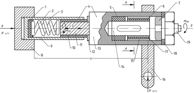
Fig. 2 shows the frictional and hydraulic parts of the damper. The reported $F_{tr}=$ 5.2 kN is an internal friction-pair force, not an external transverse track load. External excitation enters the shaft model through the loading terms and attachment motion.

Fig. 1Kinematic scheme of the patented torsion damper: 4 – torsion shaft; 8 – bogie frame; 16 – lever; 20, 26, 29 – guides; 21 – cam; 22 – car body; 23 – spherical head; 27 – splines; 28 – movable support; 30 – inclined groove

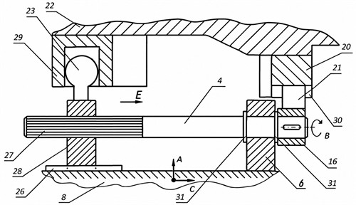
Fig. 2Longitudinal section of the hydro-friction torsion damper according to Patent IAP 07118 [8]

3. Mathematical model

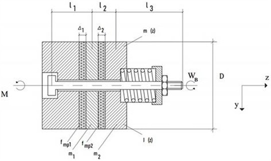
The shaft dynamics are modelled as coupled bending vibrations in two mutually perpendicular planes. Let $w_j\left(z,t\right)$ denote the transverse displacement in plane $j$, $m\left(z\right)$ the line mass (kg/m), $D_j\left(z\right)=E\left(z\right)I_j\left(z\right)$ the flexural rigidity (N·m²), $q_j\left(z,t\right)$ the external load per unit length (N/m), $r_j$ the dissipative reaction (N/m), and ${\kappa }_j$ the distributed linear restoring coefficient (N/m²). Small-deflection Euler-Bernoulli bending is assumed on each smooth segment. The calculation scheme and characteristic axial regions used in the shaft model are shown in Fig. 3. Before introducing coefficient notation, the fixed-frame balance is:

The variable-rigidity elastic operator must be expanded before division by $m\left(z\right)$:

Hence the elastic coefficients in the two displacement planes are:

Fig. 3Calculation scheme of the variable-section shaft; l1-l3 are characteristic regions and Δ1, Δ2 are friction-disc thicknesses

For constant $E$, $D_j^{\text{'}}=E{I}_j^{\text{'}}$ and $D_j^{\text{'}\text{'}}=E{I}_j^{\text{'}\text{'}}$. Thus A1 and B1 have units of m²/s², A2 and B2 have units of m³/s², and A3 and B3 have units of m⁴/s². The factor 2 in A2 and B2 follows directly from the product rule. Derivatives of $m\left(z\right)$ do not enter these elastic coefficients because the elastic operator is expanded before mass normalization.

The displacement coefficients A4 and B4 have a different physical origin and cannot be obtained from $m$, $I$ and $E$ alone. If the coordinate basis rotates at a prescribed constant angular speed $\mathrm{\Omega }$ and the restoring directions are aligned with that basis, then:

The corresponding Coriolis terms have opposite signs: $+2\mathrm{\Omega }\dot{x}$ in the y-equation and –2$\mathrm{\Omega }\dot{y}$ in the $x$-equation. The excitation angular frequency is a separate quantity and is not identified with $\mathrm{\Omega }$. For a non-rotating verification frame with no distributed restoring stiffness, $\mathrm{\Omega }=\kappa x=\kappa y=$0 and therefore $A_4=B_4=$ 0. No unmeasured rotation rate or restoring stiffness is assigned to the device.

The source model represents the variable shaft properties by sinusoidal effective-property functions before their piecewise-linear numerical approximation:

These functions are retained as the source effective-property law; assigning the same multiplier to $I$ and $m$ should not be interpreted as diameter variation alone. The source symbols $k_x$ and $k_y$ are retained only as reported effective-property functions; they are not identified with the restoring coefficient ${\kappa }_j$ without a separately defined force law and compatible units. The external dynamic excitation is represented in the source model by the harmonic-impulse form:

where $\omega$ denotes the excitation angular frequency, and $p_{0x}$ and $p_{0y}$ are the load amplitudes. Their calibrated physical values are not available in the source material.

4. Boundary conditions and numerical procedure

The shaft interval $0\le z\le L$ is divided in the source calculation into $k=$ 100 sections. Two ideal hinged supports are used at $z=$ 0 and $z=L$; transverse deflection and bending moment are zero at both ends:

The original procedure uses Fourier separation, a one-sided Laplace transform, piecewise-linear spatial coefficients, iterative eigenfrequencies, and Gaussian elimination or Cramer’s rule in Mathcad 15.

For mesh convergence, a separate spatial benchmark avoids unavailable device loads. With $\xi =z/L$ and $D_0=E{I}_0$, $D/D_0=m/m_0=1+\mathrm{s}\mathrm{i}\mathrm{n}\left(\pi \xi \right)$, simply supported ends and exact displacement $W^{*}\left(\xi \right)=\mathrm{s}\mathrm{i}\mathrm{n}\left(\pi \xi \right)$. The manufactured verification load is obtained by substitution and is not measured track excitation. Cubic Hermite meshes $N=$50, 100, 200 and 400 are compared by relative curvature-energy error eE and maximum normalized bending-moment error $eM$; the latter uses the exact maximum dimensionless moment $2{\pi }^2$.

Mesh doubling reduces both errors by approximately four, indicating second-order convergence. At $N=$100, analytical-property errors are 0.00368 % and 0.00822 %; linear interpolation gives 0.00529 % and 0.01234 %. An independent 80-term Rayleigh-Ritz calculation gives dimensionless frequencies 9.8287247, 39.2944906 and 88.7992304 versus 9.828725, 39.29449 and 88.79924 for $N=$100 Hermite elements; the maximum difference is approximately 1.1×10^-5 %. Thus $N=$100 is sufficient for this benchmark, but this does not establish mesh independence of the complete damper model.

Field observations give dominant horizontal/vertical frequencies of 3-5/7-12 Hz and piston velocities up to 520/580 mm/s in compression/rebound. They describe operating conditions but do not identify shaft load. Because synchronized transmitted-force, attachment-displacement or shaft-strain records are unavailable, the data are not used to calibrate $p_{0x}$, $p_{0y}$ or validate stresses; no quantitative attenuation, stress-reduction or fatigue-life claims are made.

The source reports heat-treated 20KhN3A limits of 430-650 MPa (normal endurance), 240-310 MPa (shear endurance), 850-1110 MPa (yield) and 950-1450 MPa (ultimate), and applies a Goodman-type assessment [14]. The required fatigue safety factor $n\ge$2 is a design requirement, not a result of this article:

The source reports a mean stiffness of 425 kN/m. Because this quantity has the units of translational stiffness, it is retained only as an equivalent assembly parameter and is not substituted for the shaft flexural rigidity EI, whose units are N·m².

5. Numerical parameters and results

The parameters directly reported in the source numerical model are summarized in Table 2.

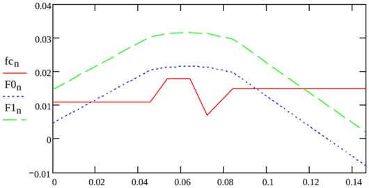
Fig. 4 compares the piecewise representation of the variable shaft-property functions from the source calculation with their spline approximation. The curves reproduce the principal spatial changes while removing discontinuities in the numerical representation. The source plot is retained only to illustrate the approximation of these functions and should not be interpreted as a stress-distribution diagram.

The former response plot is omitted because its ordinate cannot be traced to calibrated force, displacement or stress; it therefore cannot be relabelled in MPa or used to derive stress-reduction percentages.

6. Conclusions

1) The coupled two-plane shaft model is formulated with an explicitly expanded variable-rigidity operator. The elastic coefficients $A_1$-$A_3$ and $B_1$-$B_3$ follow directly from $D\left(z\right)=E\left(z\right)I\left(z\right)$ and $m\left(z\right)$; $A_4$ and $B_4$ require separately defined rotational and restoring inputs and cannot be inferred from $m$, $I$ and $E$ alone.

Fig. 4Piecewise and spline representations of the normalized variable shaft-property functions from the source calculation

2) A mesh-refinement verification of the stated variable-coefficient benchmark gives approximately second-order convergence from 50 to 400 elements. At 100 elements, the errors for analytical properties are 0.00368 % in curvature energy and 0.00822 % in sampled bending moment; with linear property interpolation, they are 0.00529 % and 0.01234 %. These values support the use of 100 subdivisions for the stated benchmark but do not establish mesh independence of the complete uncalibrated device model.

3) The source design data retained in the model include seven shaft regions, diameters of 25, 24 and 23 mm, a compressed length of 146.2 mm, a maximum length of 187.5 mm, a total damper mass of 15 kg, and an internal friction force of 5.2 kN.

4) The available frequency ranges of 3-5 Hz and 7-12 Hz and piston velocities of 520 mm/s in compression and 580 mm/s in rebound characterize operating conditions only. In the absence of calibrated transmitted loads and synchronized strain measurements, quantitative claims of stress reduction, vibration attenuation, or fatigue-life improvement are not made.