Study of the structure size interval of incomplete geometrically similitude model of the elastic thin plates

2.1. Establishment of scaling laws of the four-side simply supported elastic plate

The simply supported elastic thin plate is shown in Fig. 1. In the figure, $a$ is the length, $b$ is the width, $h$ is the thickness, $E$ is the Young's modulus, $\mu$ is the Poisson's ratio and $M_x$, $M_y$ are the bending moments.

Fig. 1Simply supported plate

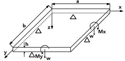
According to the Kirchhoff’s assumption, the governing equation of the thin plate can be written as [9]:

where, $D=\frac{E{h}^3}{12(1-{\mu }^2)}$, $\rho$ is the mass area ratio, $w$ is the deflection, ${\nabla }^2$is the Laplace operator, ${\nabla }^2=\frac{{\partial }^2}{\partial x^2}+\frac{{\partial }^2}{\partial y^2}$.

For the four-side simply supported plate, the boundary conditions of the Hoff theory are:

Set vibration mode function of each point as $W(x,y)$, the deflection of the plate is defined as:

Substitute Eq. (4) into Eq. (1), then the free vibration characteristics are governed by:

The scaling factor is defined as ${\lambda }_j$, where, $j$ is the symbol of physical quantities, such as $j=a,b,E,$ etc. Assuming that the model and prototype have the same materials, ${\lambda }_E=1$ then the governing equations of the model and prototype can be written as:

Eq. (6) can be written as:

Compared with Eq. (7), for the equal corresponding parameters of the equations, the following relationship can be achieved:

According to $D=\frac{E{h}^3}{12(1-{\mu }^2)}$, the following relationship can be obtained:

Substitute Eq. (10) into Eq. (9), then complete geometric similarity scaling laws of the nature frequency of the four-side simply supported elastic plates are simplified as:

For incomplete geometric similar models, ${\lambda }_a\ne {\lambda }_b\ne {\lambda }_h$, then ${\lambda }_{\omega }\ne {\lambda }_b^{-1}$, so the new scaling laws must be established. It is assumed that ${\lambda }_a=C{\lambda }_b$, where $C$ is a constant, then the scaling laws can be written as [10]:

The parameters of the prototype plate are shown in Table 1.

In order to determine geometric intervals of Eq. (12a) to Eq. (12c), it is assumed that the model and the prototype have the same materials, according to the analysis of the model shown in Table 2, to determine the approximate range of geometric intervals, namely the approximate range of $C$.

The first nature frequency of the prototype is 17.369 Hz. Based on Eq. (12a), Eq. (12b) and Eq. (12c), we can predict nature frequencies of the prototype and calculate the predicted discrepancy by using 5 kinds of models shown in Table 2, if the discrepancy $\eta \le \text{10 \%}$, the predicted values are available [11], the predicted values are shown in Table 3.

Analyzing the values shown in Table 3, the values predicted by Eq. (12b) is more accurate than the other method, so Eq. (12b) can be defined as the incomplete scaling law of the nature frequencies of elastic thin plates, and it is known that there are applicable geometric intervals within the range of M2–M4.

2.2. Analysis of the prediction discrepancy influence factors of elastic thin plates

Assuming the same materials and boundary conditions, incomplete similarity variables of elastic thin plates are the length $a$, the width $b$ and the thickness $h$. $\Gamma =a/b$, where $\Gamma$ is the relationship of length of elastic thin plates’ sides, $\Gamma >1$ for rectangular thin plates.

The formula of nature frequency of four-side simply supported elastic thin plates can be written as [8]:

where, ${\rho }_0$ is the density of the plate, $m$ and $n$ are the numbers of half waves in the plate length and width direction respectively.

According to the relationship between the model and the prototype with the same vibration mode shape, we obtain:

The nature frequency of the model is represented as:

Multiply Eq. (15) by Eq. (12b), we can obtain:

The predicted discrepancy of incomplete geometric similarity can be defined as:

Substitute Eq. (14), Eq. (16) into Eq. (17), which can be simplified as:

According to Eq. (18), the following conclusions can be obtained:

(1) ${\lambda }_h\mathrm{}$is independent, namely ${\lambda }_h$ has no effect on the predicted discrepancy of incomplete geometric similarity;

(2) ${\lambda }_b$ has no effect on the predicted discrepancy of incomplete geometric similarity, but $C={\mathrm{\lambda }}_a/{\mathrm{\lambda }}_b$ does;

(3) The size parameters of prototype $a,b$ has no effect on incomplete geometric similarity applicable intervals, $\Gamma =a/b$ has effect on the intervals and mode shapes.

From above conclusions, we know that the geometric applicable intervals of simply supported elastic thin plates is the range of $C$ under different $\Gamma$ by using Eq. (12b) as the scaling law.

3.1. Structure size intervals of the first-order nature characteristics

3.1.1. Applicable geometric intervals of distorted plate models

The geometrical parameters of the prototype plate: $a=\Gamma b$, $b=\text{10 m}$, $h=\text{0.5 m}$, ${\lambda }_b={\lambda }_h=20$, its material parameters are shown in Table 1. From the three above conclusions, we know that the analysis has general applicability by using the prototype.

Assuming $\Gamma =a/b=1.05$, according to ANSYS calculation, the first-order nature frequency is ${\omega }_p=\text{23.092 Hz}$.

The first-order nature frequency ${\omega }_{pr}^1$ is respectively predicted as six discrete values $C=\left[0.6,\mathrm{}0.7,\mathrm{}0.95,\mathrm{}1.3,\mathrm{}1.65,\mathrm{}1.95\right]\text{,}$ then the relationship between the first-order natural frequencies and $C$ is obtained by fitting a fourth order polynomial:

19

${\omega }_{pr}^1=6.34C^4-39.26C^3+93.5C^2-95.68.$

Verify the curve by other discrete values in the range of $C$, the step size of which is 0.05, and they fit the curve well, as shown in Fig. 2.

Fig. 2Verification of fourth-order polynomial fitting results

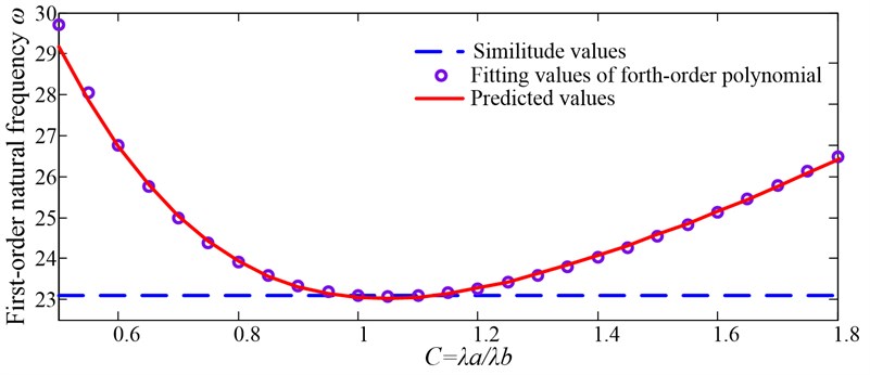
From Fig. 2, we know that Eq. (19) has accurate fitting effects in the range of $C\in \left[0.6,1.95\right]$.By introducing a ±10 % discrepancy of $\eta$, the acceptable range of $C$ are calculated as:

20

$\eta =\frac{\left|（6.34C^4-39.26C^3+93.5C^2-95.68C+58.14-23.09）\right|}{23.09}=0.1.$

The roots of Eq. ($20$) under the intervals $C\in [0.6,\mathrm{}1.95]$ are $C_{min}=0.675$ and $C_{max}=1.646$. So, when $\Gamma =a/b=1.05$, the applicable geometric interval is $C\in [0.675,\mathrm{}1.646]$.

3.1.2. Boundary function

Calculating values of $C_{min}$ and $C_{max}$ under the corresponding $\Gamma =[1,1.1,\mathrm{}1.15,\mathrm{}1.225]$ by using the above method, as shown in Table 4, the fitting polynomial curves are shown from Fig. 3 to Fig. 6. The maximum value of 1.225 is based on the control intervals of shape modes in higher-order frequencies’ prediction below.

Fig. 3Fitting curve of Γ=1.0

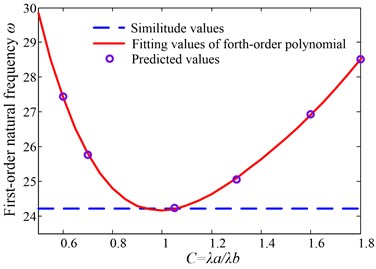
Fig. 4Fitting curve of Γ=1.1

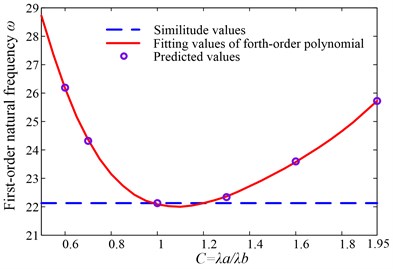
Fig. 5Fitting curve of Γ=1.15

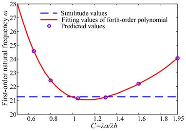
Fig. 6Fitting curve of Γ=1.225

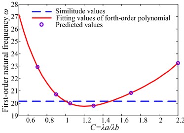
Table 4Interval boundary values with different Γ

	$\Gamma =$1.0	$\Gamma =$ 1.1	$\Gamma =$ 1.15	$\Gamma =$ 1.225
Fourth order polynomial equations	$8.04C^4-47.24C^3+107C^2-104.2C+60.6$	$6.69C^4-41.02C^3+96.61C^2-98.93C+58.73$	$5.84C^4-36.44C^3+87.64C^2-92.34C+56.52$	$3.85C^4-26.19C^3+68.59C^2-78.24C+52.16$
Frequencies of the prototype / Hz	$24.22$	$22.12$	$21.27$	$20.18$
Boundary values	$C_{min}=0.644,$ $C_{max}=1.55$	$C_{min}=0.702,$ $C_{max}=1.741$	$C_{min}=0.723,$ $C_{max}=1.855$	$C_{min}=0.753,$ $C_{max}=2.028$

From the boundary values of $\Gamma =1.05$ and the values shown in Table 4, we know:

21

$\left\{\begin{array}{l}\Gamma =\left[\mathrm{1.0,1.05,1.1,1.15,1.225}\right],\\ C_{min}=\left[\mathrm{0.644,0.675,0.702,0.723,0.753}\right],\\ C_{max}=\left[\mathrm{1.55,1.646,1.741,1.855,2.028}\right].\end{array}\right.$

By using fitting third-order polynomial, $C_{min}$ and $C_{max}$ can be written as:

22

$C_{min}=2.38{\Gamma }^3-8.62{\Gamma }^2+10.81\Gamma -3.93,$

23

$C_{max}=-0.96{\Gamma }^3+4.65{\Gamma }^2-4.664\Gamma +2.52.$

The functional curves of Eq. (22) and Eq. (23) are shown in Fig. 7.

Fig. 7Boundary values of structure size applicable intervals

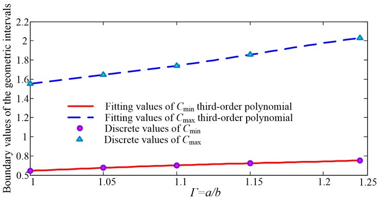
In Fig. 7, the area among the two cures is the applicable geometric intervals of first-order nature frequency of simply supported plates in the range of $\Gamma \in (1,1.225)$.

3.2. Structure size intervals of the higher-order nature characteristics

The geometric size distortion will cause the jump of thin plate models’ mode shapes, for the prototype in this paper, it is assumed that the range of size which can keep the same mode shapes between the model and the prototype is $\Gamma \in (1,{\Gamma }_j]$, as shown in Table 5.

According to ${\lambda }_b=C{\lambda }_a$, the ratio of the length to the width of the plate model is:

For satisfying the prediction accuracy of higher-order nature frequencies of the plate model, and keeping the same mode shapes between the model and the prototype, so the model size is satisfied as:

where, $j$ represents the order number of nature frequency.

According to Eq. (24) and Eq. (25), the applicable geometric intervals of higher-order nature frequencies of the distorted model is:

where, $\left[C_{min}^j\left(\Gamma \right),C_{max}^j\left(\Gamma \right)\right]$is the predicted intervals of higher-order nature frequencies, $\left[\Gamma /{\Gamma }_j,\Gamma \right)$ is the mode shape control intervals of the prototype in this paper, their intersection is the applicable geometric intervals of higher-order nature frequencies in $\Gamma \in (1,{\Gamma }_j]$.

According to actual requirements, the range of $\Gamma$ is chosen based on different principles, so the range of each size is different, in this paper, choosing the mode shape control intervals based on the same first 8 modes, so ${\Gamma }_8=1.225$.

It is different from the first-order nature frequency that the mode shapes of higher-order nature frequencies will change along with the change of $C$, and it is difficult that $C_{min}^j\left(\Gamma \right)$ and $C_{max}^j\left(\Gamma \right)$ are obtained by using low-order polynomial fitting, considering the boundary values of applicable geometric intervals are the intersection of the predicted intervals of higher-order nature frequencies and the mode shape control intervals, so when analyzing the geometric intervals of higher-order nature frequencies by numerical method, the $C$ value of the plate model satisfies $C\in \left[\Gamma /{\Gamma }_j,\Gamma \right)$, solving the applicable geometric intervals of the fifth-order nature frequency of the prototype, as shown in 4.1.1.

Choosing $\Gamma =[1,\mathrm{}1.05,\mathrm{}1.1,\mathrm{}1.15,\mathrm{}1.225]$, calculating the boundary values of the applicable geometric intervals by interpolation method, as shown in Table 6.

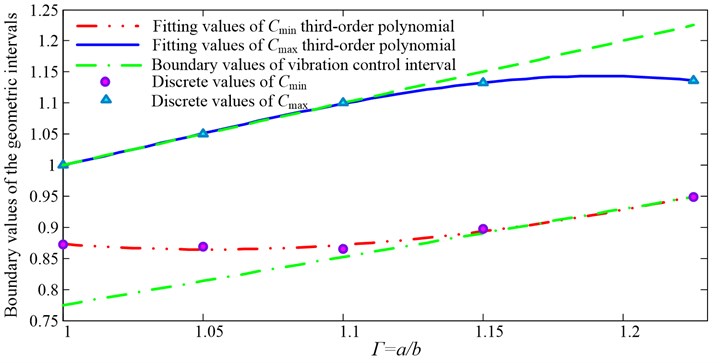
According to the data shown in Table 6, we obtain:

By using fitting third-order polynomial, $C_{min}$ and $C_{max}$ can be written as:

The functional images of Eq. (22) and Eq. (23) are shown in Fig. 8.

Fig. 8The fifth-order boundary values of structure size applicable intervals

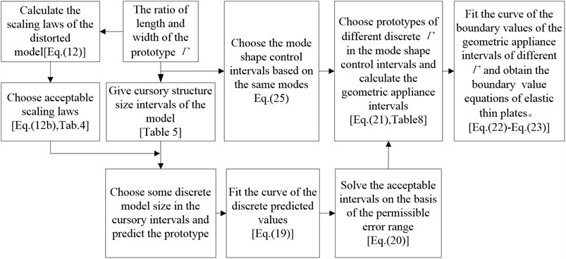
4.1. The flow of determination method

The flow chart about determination of geometric applicable intervals of elastic thin plates’ similar models is shown in Fig. 9.

4.2. Experiment

For the accuracy of the scaling laws and the intervals determination method, choose the titanium alloy single layer plates with same materials and different sizes as the experimental models, their parameters of materials and structural sizes are shown in Table 7.

The ratio of length to width of the prototype is $\Gamma =1.136$, that of the model is $\Gamma =1.125$, $C=1.01$, in the applicable geometric intervals, the values of nature frequencies of the prototype and the model, and the predicted discrepancy are shown in Table 8.

From Table 8, we know that the predicted values of the model are accurate in applicable geometric intervals, and it is verified that the applicable geometric intervals are valid for the design of similar models.