Application of sound loudness research in structural-acoustic coupling cavity with impedance and mobility approach method

1. Introduction

The sound quality of machine elements is of great importance in the design of high-quality machinery. Noise in an enclosed cavity, such as in the interior car, has been paid more attention in recent years. Therefore, it is particularly significant to control the sound quality in an enclosed cavity. Among the parameters of sound quality, loudness is a very important parameter.

Many researchers have studied noise in an enclosed cavity by using Finite Element Method (FEM) since 1960s. Gladwell and Zimmermann developed an energy formulation of the structural-acoustic theory, in which the stage was set for the application of FEM to acoustic cavity analysis [1]. Early contributions to development of finite element approach were made by Craggs [2], Shuku and Ishihara [3], primarily providing a practical method for analyzing the acoustic of the automobile passenger compartment. And NASTRAN was used by Nefske and Wolf [4] for the study of automobile interior noise, as well as its application into structural-acoustic analyses of the passenger compartment was described.

As for the calculation of sound loudness, on the basis of Zwicker’s loudness model [5], researchers have provided some methods such as EMBSD [6], PSQM [7], PEAQ [8] and etc. However these methods still fail to provide all of the necessary details. These have been summarized in [9]. Then Kabla [10] corrected the PEAQ method which was more precise than the others. In the present paper, the corrected PEAQ approach is applied to calculate the sound loudness radiated from rectangular acoustic-structure coupling plates.

The impedance and mobility approach method for the analysis of structural-acoustic systems was proposed by Kim in 1999 [11]. The kernel idea is derived acoustic mode amplitude contribution and elastic plate mode amplitude contribution in cavity by using cavity impedance $Z_n$, the structural mobility $Y_s$, modal coupling coefficients $C_{n,m}$ of modal synthesis theory.

Consequently, the sound loudness in an enclosed cavity is thus calculated. By comparing the different location point in the structural-acoustic coupling cavity with a harmonic force excitation on an elastic plate and taking the frequency selectivity of human hearing system into account, the effects of sound loudness are studied in detail.

2. Zwicker’s sound loudness model

The sensation that corresponds most closely to the sound intensity of the stimulus is loudness. Critical bandwidth plays an important role in the loudness, and the loudness on the slopes of the frequency selectivity characteristic of human hearing system may also play an important role. The excitation level versus critical-band rate represents the pattern that describes not only the influence of critical bandwidth but also that of the slopes. Therefore, it seems reasonable to use the excitation level versus critical-band rate as a basis from which the complex of the loudness may be constructed [13]. The loudness is then an integral of the specific loudness over all critical-band rates [5]:

Thus, the transformation from critical-band rate level into excitation level versus critical-band rate is necessary. Both the frequency related transformation into critical-band rate and amplitude related transformation into specific loudness are of crucial importance for evaluating sound at the specific receiver, e.g. the human hearing system. The transformation from excitation level into specific loudness must be known in order to transform excitation level versus critical-band rate into specific loudness versus critical-band rate. This transformation is discussed below.

Steven’s law [14] says that a sensation belonging to the category of intensity sensations grows with physical intensity according to a power law. According to this law, one has to assume that a relative change in loudness is proportional to a relative change in intensity. Instead of the total loudness, specific loudness is used as the value. According to the Zwicker’s loudness model, the specific loudness is given by as follows [5]:

where $E_{TQ}$ is the excitation level at the threshold in quiet approximated by $E_{TQ}\left(f\right)=3.64{\left(f/1000\right)}^{-0.8}$, $E_0$ is the excitation corresponding to the reference intensity $I_0={10}^{-12}W/m^2$. The values for these two parameters are given in [10].

The critical-band concept is thus important to describe human hearing sensations. And the concept of critical-band rate scale is derived, which is based on the fact that human hearing system analyses a broad spectrum into parts that correspond to critical bands. In many cases, an analytic expression is useful to describe the dependence of the critical-band rate (and of the critical bandwidth) on the frequency over the whole auditory frequency range. The following relations are useful [5]:

and:

where $z$ is critical-band rate, $\Delta f_G$ is critical bandwidth.

The frequency selectivity of human hearing system can be approximated by subdividing the intensity of the sound into parts that fall into critical band. In order to describe such approximation, the notion of critical-band intensities is put forward. The critical-band level and the excitation level play an important role in many acoustic models. The critical-band level intensity $I_G$ can be calculated from the following equation that takes into account the frequency dependence of critical bandwidth [5]:

The critical-band rate $z$ is useful in describing the characteristics of human hearing system. Because the critical-band rate $z$ is a definite function of frequency, $I_G$ can also be expressed in terms of the critical-band rates:

In logarithmic scale, using $I_0={10}^{-12}\text{W/}{\text{m}}^{\text{2}}$ as reference value, the critical-band level $L_G$ is defined as:

The critical-band intensity can be seen as that part of the overall unweighted sound intensity which falls within a frequency window that has the width of a critical band. The transformation of the frequency into the critical-band rate transfers the frequency-dependent window width into a window width of 1 Bark, independent of the critical-band rate. Consequently, a critical-band wide narrow-band noise produces a critical-band intensity which is a function of the critical-band rate, and which shows the form of a triangle with a base width of 2-Bark. A harmonic tone, however, produces a function with a rectangular shape and the width of 1 Bark.

The intermediate values such as the excitation or the excitation level, however, represent a much better approximation to the frequency selectivity of human hearing system. The so-called main excitation corresponds in this transformation to the maximum value of the critical-band level. In most cases, the excitation level, defined by $L_E$, is given by [5]:

The excitation level can be constructed most simply from the critical-band level as a function of the critical-band rate, by calculating the critical-band level in the range of the main excitation. In cases of an abrupt change of the intensity density as a function of the critical-band rate, as for low-pass noise or sinusoidal tones, the excitation level is identical to the critical-band level.

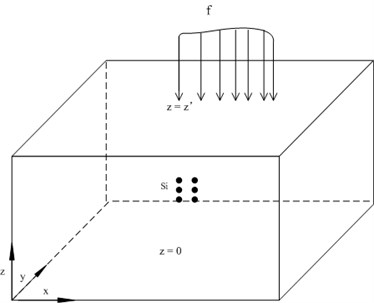
Fig. 1Sketch map of structural-acoustic coupling cavity including force excitation distribution and sound intensity excitation

3. Model of impedance and mobility approach method

The impedance and mobility approach method for the analysis of structural-acoustic systems was proposed by Kim in 1999 [11]. The kernel idea is derived acoustic mode amplitude contribution and elastic plate mode amplitude contribution in cavity by using cavity impedance $Z_n$, the structural mobility $Y_s$, modal coupling coefficients $C_{n,m}$ of modal synthesis theory. This article analyses regularities of loudness distribution in cavity which has six elastic plates with simple support.

Think about a rectangle structural-acoustic coupling cavity, as shown in Figure 1.

In cavity there is full of air whose density is ${\rho }_a$, and all boundary plates are elastic with simple support. There are a force distribution function $f(\omega ,L_p)$ on plate $z=z\text{'}$ and a sound intensity function $si(\omega ,L_c)$ in the structural-acoustic coupling cavity. Let’s suppose coupling response could be decomposed into limited uncoupled acoustic modes and structural modes, and these uncoupled modes are acoustic modes cavity with rigid walls and structural modes in vacuum. There are $n$-th acoustic modes and $m$-th structural modes. Therefore, sound pressure $p$ at point $L_c$ is as follows:

where $n$-dimensional column vector $\mathbf{\Psi }$ represents uncoupled acoustic modes shape function ${\psi }_n\left(x\right)$ and $n$-dimensional column vector $\mathbf{a}$ represents sound pressure modes complex amplitude, sign $T$ at top left corner means transposition. The acoustic modes shape function ${\psi }_n\left(x\right)$ is orthogonal in each uncoupled cavities as follows:

where $V$ represents the volume of acoustic cavity. According to reference [11], since all boundary plates are simple support elastic plates, the relations between $n$-th sound pressure modes amplitude and external excitation is as follows:

where, ${\rho }_a$ represents air density in cavity, $c_a$ represents sound speed in air, two integral expressions in the bracket represent $n$-th acoustic modal intensity caused by $si(L_c,\omega )$ and $u\left(L_{pSi},\omega \right)$. $u\left(L_{pSi},\omega \right)$ represents the vibration velocity of each simple support elastic plate which surround the cavity, as shown bellow:

where, $m$-dimensional column vector $\mathbf{\Phi }$ represents uncoupled vibration shape modal function ${\varphi }_m\left(y\right)$ and $b$ represents uncoupled vibration velocity modal complex amplitude $b_m\left(\omega \right)$. The modal shapes functions ${\psi }_n\left(x\right)$ and ${\varphi }_m\left(y\right)$ are orthogonal in each uncoupled system, and the expression is as below:

Then $a$ is shown as below:

where $r_n={\int }_V{\psi }_n\left(L_c\right)si(L_c,\omega )dV$, the acoustic modal resonant expression $A_n\left(\omega \right)$ is as below:

where $T_a$ represents time constant of first modal, ${\omega }_n$ represents $n$-th acoustic modal frequency, ${\zeta }_n$ represents $n$-th acoustic modal damping factor. $C_{n,m}^i$ represents coupled relations between the $i$-th uncoupled plate and acoustic modal shape function, which is as follows:

Then $a$ could represent as follows:

where, $\mathbf{r}$ represents $n$-th modal source intensity vector, ${\mathbf{q}}_s=\sum {\mathbf{C}}^{i}b$ represents source intensity vector caused by elastic structural vibration, whose effect is a group of external sound source function in elastic structure. $b$ is $m\text{th}$ amplitude modal vector, $\mathbf{C}$ is $(n\times m)$ dimension structural-acoustic modal shape function coupled matrix. ${\mathbf{Z}}_a=\raisebox{1ex}{$A{\rho }_a{c}_a^2$}\!\left/ \!\raisebox{-1ex}{$V$}\right.$ which composed by $(n\times n)$ dimension uncoupled acoustic modal impedance diagonal matrix.

The $m$-th modal amplitude of the plate $z=z\text{'}$ is as follows:

where ${\rho }_s$ represents density of plate, $h_{z\text{'}}$ represents thickness of plate, $S_{z\text{'}}$ represents area of the plate $z=z\text{'}$, $p(L_{pSz\text{'}},\omega )$ represents sound pressure distribution function affected on the plate $z=z\text{'}$. The first and the second integral formulae in the expression represent $m$-th vibration modal forces caused by $f(L_{pSz\text{'}},\omega )$ and $p(L_{pSz\text{'}},\omega )$. The minus between two integral formulae is because of the opposite directions of external forces and acoustic pressure forces.

Similarly, the $m$-th modal vibration amplitude of the other elastic plate without external forces is as below:

where, $h_i$ represents thickness of plate, $S_i$ represents area of plate $i$.

The resonant term of plate could be expressed as follows:

where ${\omega }_m^i$ represents $m$-th modal frequency of plate $i$, ${\zeta }_m^i$ represents $m$-th modal damping ratio of plate $i$.

The modal vibration amplitude contribution vector of plate $z=z\text{'}$ is as follows:

The modal vibration amplitude contribution of the other plates is:

where ${\mathbf{C}}_{n,m}^{iT}={\mathbf{C}}_{m,n}^i$. Consequently, the modal vibration amplitude vector of plate $z=z\text{'}$ is as below:

where $m\text{-dimensional}$ vector $\mathbf{F}$ is caused by external load distribution function $f(L_{pz\text{'}},\omega )$, $g_a={{\mathbf{C}}^{z\text{'}}}^{T}a$ represents modal force vector affected on acoustic cavity system, which is the elastic plate structural reaction exciting by acoustic pressure fluctuation. ${\mathbf{Y}}_s^{z\text{'}}=\raisebox{1ex}{${\mathbf{B}}^{z\text{'}}$}\!\left/ \!\raisebox{-1ex}{${\rho }_s{h}_{z\text{'}}{S}_{z\text{'}}$}\right.$ represents modal mobility diagonal matrix of plate $z=z\text{'}$.

The modal vibration amplitude contribution vector of other plates is as below:

Where $g_a={{\mathbf{C}}^i}^{T}a$ represents modal force vector affected on acoustic cavity system, which is the elastic plate structural reaction exciting by acoustic pressure fluctuation. ${\mathbf{Y}}_s^i=\raisebox{1ex}{${\mathbf{B}}^i$}\!\left/ \!\raisebox{-1ex}{${\rho }_s{h}_i{S}_i$}\right.$ represents modal mobility diagonal matrix of other plates. Similar to acoustic impedance matrix ${\mathbf{Z}}_a$, ${\mathbf{Y}}_s^{z\text{'}}$ and ${\mathbf{Y}}_s^i$ are also diagonal matrixes.

According to the derivation above, the formula is shown as below after uncoupling:

The equation above could be adapted into impedance-mobility form. Suppose there is only one force excitation on plate $(\mathbf{r}=0)$, and put $q_s=\sum {\mathbf{C}}^{i}b$ into $\mathbf{a}={\mathbf{Z}}_a(\mathbf{r}+{\mathbf{q}}_s)$, then $a=\sum {\mathbf{Z}}_a{\mathbf{C}}^{i}b$ could be obtained. $g_a={{\mathbf{C}}^i}^{T}a$ is combined with $a=\sum {\mathbf{Z}}_a{\mathbf{C}}^{i}b$, the following equation is obtained:

where ${\mathbf{Z}}_{ca}^i={{\mathbf{C}}^i}^T{\mathbf{Z}}_a{\mathbf{C}}^i$ represents coupled acoustic modal impedance diagonal matrix. Similarly, ${\mathbf{Y}}_{cs}^i={\mathbf{C}}^i{\mathbf{Y}}_s^i{{\mathbf{C}}^i}^T$ can be defined as coupled structural modal mobility diagonal matrix. Therefore, $\mathbf{a}={\left(\mathbf{I}+{\mathbf{Z}}_a\sum {\mathbf{C}}^i{\mathbf{Y}}_s^i{{\mathbf{C}}^i}^T+{\mathbf{Z}}_a{\mathbf{C}}^{z^{\text{'}}}{\mathbf{Y}}_s^{z^{\text{'}}}{\mathbf{C}}^{z^{\text{'}}T}\right)}^{-1}{\mathbf{Z}}_a\left(\mathbf{r}+{\mathbf{C}}^{z^{\text{'}}}{\mathbf{Y}}_s^{z^{\text{'}}}\mathbf{F}\right)$ can be rewritten as follows:

Since the structural mobility ${\mathbf{Y}}_s^{z\text{'}}$ and coupling coefficient ${\mathbf{C}}^{z\text{'}}$ of plate $z=z\text{'}$ is the same with plate $z=0$, the equation above can be derived as follows:

The equation above is the compact calculation form of classic theory on acoustic modal contribution about the coupling response, which is in the field of structural-acoustic coupling system with both structural force excitation and acoustic source excitation.

According to reference [11], the standard evaluation criterion for weak coupling, the acoustic response $[\mathbf{I}+{\mathbf{Z}}_a{\mathbf{Y}}_{cs}]\approx \left[\mathbf{I}\right]$. That is to say, ${\mathbf{Z}}_a{\mathbf{Y}}_{cs}$could be almost equals 0 in the equation $\mathbf{a}={\left(\mathbf{I}+{\mathbf{Z}}_a\sum {\mathbf{Y}}_{cs}^i+{\mathbf{Z}}_a{\mathbf{Y}}_{cs}^{z^{\text{'}}}\right)}^{-1}{\mathbf{Z}}_a\left(\mathbf{r}+{\mathbf{C}}^{z^{\text{'}}}{\mathbf{Y}}_s^{z^{\text{'}}}\mathbf{F}\right)$ in weak coupling system, therefore, the follows can be obtained:

Put $\mathbf{a}={\mathbf{Z}}_a(\mathbf{r}+{\mathbf{C}}^{z\text{'}}{\mathbf{Y}}_s^{z\text{'}}\mathbf{F})$ into $p\left(L_c,\omega \right)=\sum _{n=1}^N{\psi }_n\left(L_c\right)a_n\left(\omega \right)={\mathbf{\Psi }}^T\mathbf{a}$, the sound pressure value of some node in the acoustic-structural coupling field could be calculated as below:

4. An example

According to the models above, the distribution of sound loudness in the rectangle enclosed acoustic-structural coupling field under the condition of one excitation on one elastic plate is studied.

Fig. 2Structural-acoustic rectangle system with one harmonic force excitation

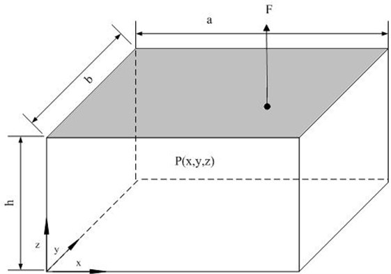
Figure 2 is a rectangle cavity which is composed by five rigid walls and one elastic plate with simple support on its boundary, $a=$ 0.5 m, $b=$ 0.4 m, $h=$ 0.3 m. In the cavity there is fill with air, its density is ${\rho }_0=$ 1.225 kg/m³. The sound velocity is $c=$ 340 m/s. The density of plate is ${\rho }_s=$ 2790 kg/m³, the thickness is 5 mm, Poisson ratio is $v=$ 0.3, the modulus of elasticity is $E=$ 70×10⁹ N/m², the damping loss factor is $\xi =$ 0.01. The coordinate of the excitation point is (0.4, 0.1, 0.3), the excitation force is $f=e^{j\omega t}\left(N\right)$, which range is from 1 Hz to 630 Hz.

The natural frequency and natural mode of each order of the elastic plate are as below:

which $L_1\times L_2$ is the length and width of the elastic plate, $m_1$ and $m_2$ are positive integers, $D=E{h}^3/\left[12\rho \right(1-{\mu }^2\left)\right]$ represents bending rigidity, $\rho$ represents density of aluminum, $h$ represents thickness of the plate, $\mu$ represents Poisson ratio.

The natural frequency and natural mode of each order of the rectangle cavity are as below:

where $L_1\times L_2\times L_3$ represents the size of the rigid walls, if $n_i=0$, then $e_i=1$; else $e_i=2$, $i=\mathrm{1,2},3$.

According to (30) and (32), the response natural frequencies of each order of the plate and cavity is shown in Table 1 and Table 2.

According to reference [15], the modal coupling coefficient of this example can be represented as below:

The ratio loudness at cross section $z=$ 0.15 m which frequency is 125 Hz, 250 Hz and 450 Hz are shown in Fig. 3.

According to Figure 3, the ratio loudness distribution changes greatly in different frequencies. When the frequency is 125 Hz, the minimum ratio loudness point is at point (0.1, 0.1, 0.15). Regard this point as original point, it can be found that the increasing speed of ratio loudness along $x$ direction is obviously faster than $x$ direction. But the variation range at 125 Hz is smaller than higher frequency.

When the frequency is 250 Hz, the minimum ratio loudness point is at point (0.45, 0.15, 0.15) and its value is only 14 sone/Hz. Except for the minimum ratio loudness point, there are other low ratio loudness points such as point (0.45, 0.3, 0.15), (0.28, 0.36, 0.15), (0.18, 0.4, 0.15) and (0.11, 0.044, 0.15).

Fig. 3Ratio loudness diagrams where cross section z= 0.15 m

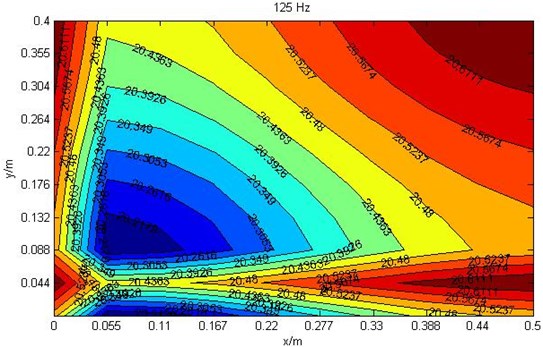
a) Ratio loudness diagram at 125 Hz where cross section $z=$ 0.15 m

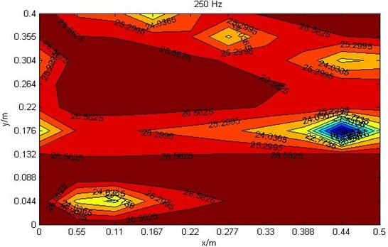
b) Ratio loudness diagram at 250 Hz where cross section $z=$ 0.15 m

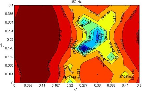
c) Ratio loudness diagram at 450 Hz where cross section $z=$ 0.15 m

When further increasing of frequency to 450 Hz, the ratio loudness value is also increasing, but its distribution shape is greatly changed from the 250 Hz shape. Its minimum ratio loudness value is 32.5 sone/Hz which is at point (0.35, 0.2, 0.15) and point (0.275, 0.175, 0.15). The average ratio loudness value is 36 sone/Hz which is obviously higher than the frequency 250 Hz.

Three observation points whose coordinates $o{b}_1$ (0.055, 0.044, 0.15), $o{b}_2$ (0.275, 0.176, 0.25) and $o{b}_3$ (0.33, 0.22, 0.15) are chosen to study their variation law.

Fig. 4Curves of sound intensity level at three different observation points

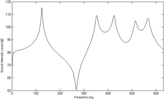
a) Curve of sound intensity level at point $o{b}_1$

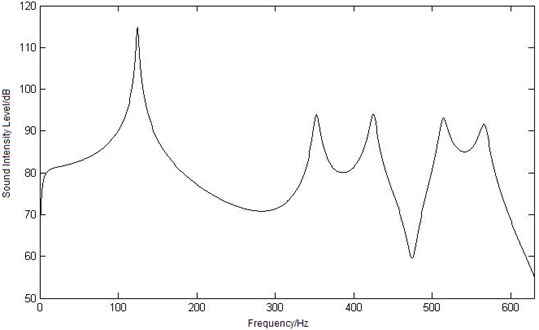
b) Curve of sound intensity level at point $o{b}_2$

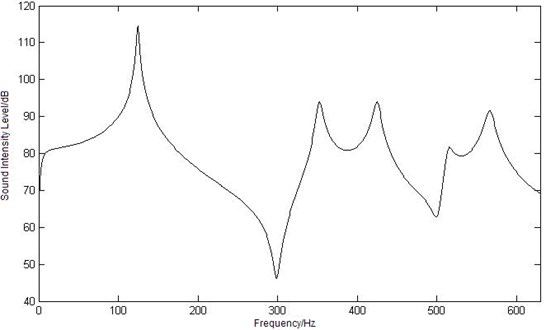
c) Curve of sound intensity level at point $o{b}_3$

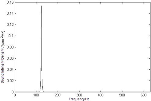
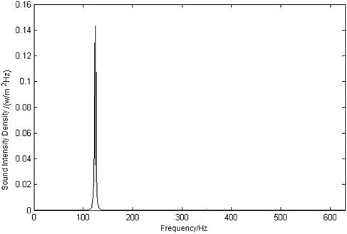
Fig. 5Curves of sound intensity density at three different observation points

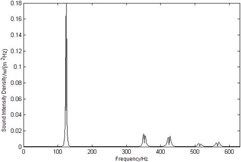
a) Curve of sound intensity density at point $o{b}_1$

b) Curve of sound intensity density at point $o{b}_2$

c) Curve of sound intensity density at point $o{b}_3$

The sound intensity level curve of the three observation points $o{b}_1$, $o{b}_2$, $o{b}_3$ is shown as Figure 4. Compare in the figure, a similar tendency of all these curves can be seen: the maximum sound intensity level values appear when the frequency is 125 Hz, and as the first order mode frequency of the elastic plate is 124.64 Hz, it can be concluded that the maximum sound intensity level value is caused by the first order mode frequency. And with the increasing of frequency, the intensity level value decreases until the second maximum value appears at 355 Hz. The value of sound intensity level is oscillating and three peak values is obtained at 425 Hz (the 8th order mode frequency of the cavity), 510 Hz and 567 Hz (the 13th order mode frequency of the cavity). But there are great differences with the sound intensity level curves of three observation points: the minimum sound intensity level value of point $o{b}_1$ is 50.5 dB at 268 Hz, which point $o{b}_2$ is at 630 Hz, point $o{b}_3$ is at 299 Hz. According to the three curves, a conclusion can be drawn that the first order mode of elastic plate has made great contributions to the coupling intensity level in low frequency range, and the mode of cavity make more in middle and high frequency area.

Because of the frequency selectivity of human hearing system, the sound intensity density $dI/df$ is important in the process of estimating the sound loudness. According to the sound loudness model that has been set up in section 2, the sound intensity density $dI/df$ can be calculated as shown in Fig. 5.

In Figure 5, the maximum value of the observation points’ sound intensity density in enclosure coupling cavity is relative to the maximum sound intensity level value, that is to say, the first mode frequency has made great contribution to the acoustic-structural coupling cavity.

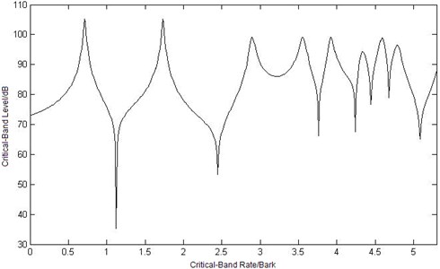
Since the critical-band rate scale is better to describe human hearing sensations and the critical-band rate $z$ is a definite function of frequency, the sound intensity density $dI/df$ can be expressed as $dI/dz$ by using the critical-band rate scale according to Equation (3). Once the sound intensity density $dI/dz$ is obtained, then the critical-band level intensity $I_G$ can be calculated according to Equation (6). Thus, at the observation point, one can obtain the critical-band level $L_G$ caused by different observation place is as shown in Fig. 6.

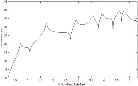
Because of the frequency selectivity of human hearing system, there are more local maximum or minimum values of critical-band level curves under critical-band rate scale in Figure 6, which is different from sound intensity level curves in Figure 4. So does the differential value between the maximum value and the minimum value. The three critical-band level curves have the same trend except the differential range in Figure 6. But when the value of the abscissa of critical-band level is greater than 3 Bark, there is obviously difference in the curves, which is not the same with the trend of sound intensity level in Figure 4.

The excitation level at threshold in quiet has different value at different frequency because of the frequency selectivity of human hearing system, which is shown in Fig. 7. For this characteristic of human hearing system, the sound loudness obtained at the observation point has low value in low frequency range as shown in Fig. 8. On the other hand, though the effect of thickness on the sound loudness is similar to the effect on the critical-band level, there are still great differences.

Equation (2) is one of the most sophisticated specific loudness calculation methods [6]. The power spectrum of each frame is weighted by the frequency selectively of the human hearing. The power spectral energies are then grouped into critical bands. An offset is then added to the critical band energies to compensate for internal noise generated in the ear. Because the sound at the observation is harmonic tones, according to Equations (1) and (2) and the transformation of the excitation level from the critical-band level described in section 2, the sound loudness at the observation point is calculated as shown in Fig. 8.

In Figure 8, loudness of point $o{b}_1$ is higher than the other observation points, and significant difference can be seen when the critical-band is in middle and high frequency (greater than 3.8 Bark). In low-frequency area, the shapes of the loudness curve are similar because the modes of elastic plate play a major role to the loudness values, although the observation points are in different location. With frequencies arising, the modes of cavity play an increasingly important role to loudness values. So the distribution location in the cavity appears to have more effect to loudness values in middle-high-frequency range. In the three observation point, the length of point $o{b}_2$ and $o{b}_3$ to the exciting point is nearer than the one of point $o{b}_1$, but loudness value of point $o{b}_1$ is the higher than the other two points. That is to say, loudness in the cavity is irrelevant to the distance to exciting point.

Fig. 6Curves of critical-band level at three different observation points

a) Curve of critical-band level at point $o{b}_1$

b) Curve of critical-band level at point $o{b}_2$

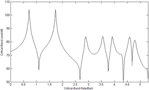
c) Curve of critical-band level at point $o{b}_3$

Fig. 7Excitation level of human hearing threshold

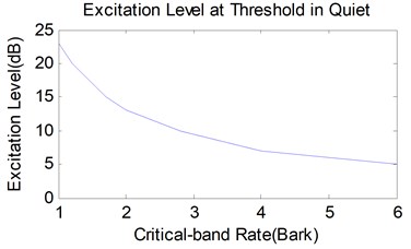
Fig. 8Curves of sound loudness at three different observation points

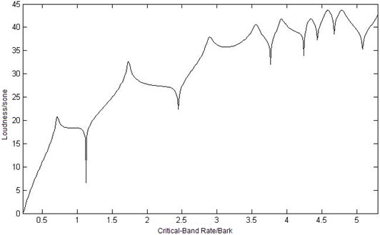
a) Curve of sound loudness at point $o{b}_1$

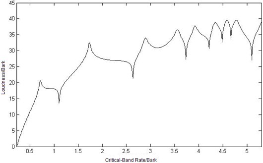
b) Curve of sound loudness at point $o{b}_2$

c) Curve of sound loudness at point $o{b}_3$

5. Conclusions

Based on the theory of impedance and mobility approach method, this paper has improved the application of structural-acoustic coupling model of this theory. The distribution of sound loudness in the rectangle enclosed acoustic-structural coupling field under the condition of one excitation on one elastic plate is studied. Because of the frequency selectivity of human hearing system, the characteristics of sound loudness are greatly different from the sound intensity level obtained in the cavity. The different location of observation points has different sound loudness and the sound intensity level. When taking the frequency selectivity of human hearing system into account, the critical-band level and the sound loudness in the enclosed cavity illustrate well the influence of human hearing frequency characteristic on human sensation. The result of this study shows:

(1) The distribution of the sound loudness is NOT even in the cavity in different frequency and different locations, but they have a similar distribution rule.

(2) In low-frequency range, the main contribution to sound loudness in the cavity is elastic plate mode, with the increase of frequency, the main contribution is the cavity acoustic mode in middle-high-frequency.