Dynamic response of a pavement-subgrade-soft ground system subjected to moving traffic load

Lu, Zheng; Yao, Hailin; Liu, Jie; Hu, Zhi

Journal of Vibroengineering

Browse Journal

Submit article

Published: 15 February 2014

Check for updates

Dynamic response of a pavement-subgrade-soft ground system subjected to moving traffic load

Zheng Lu¹

Hailin Yao²

Jie Liu³

Zhi Hu⁴

^{1, 2, 3, 4}State Key Laboratory of Geomechanics and Geotechnical Engineering Institute of Rock and Soil Mechanics, Chinese Academy of Sciences, Wuhan 430071, China

Corresponding Author:

Zheng Lu

Cite the article Download PDF

Downloads 1187

WoS Core Citations 14

Abstract

This paper introduces a three-dimensional model for the steady-state response of a pavement-subgrade-soft ground system subjected to moving traffic load. A semi-analytical wave propagation model is introduced which is subjected to four rectangular moving loads and based on a calculation method of the dynamic stiffness matrix of the ground. In order to model a complete road system, the effect of a simple road model is taken into account including pavement, subgrade and soft subsoil. The pavement and the subgrade are regarded as two elastic layers resting on a poroelastic half-space soil medium. The priority has been given to a simple formulation based on the principle of spatial Fourier transforms compatible with good numerical efficiency and yet providing quick solutions. The frequency wave-number domain solution of the road system is obtained by the compatibility condition at the interface of the structural layers. By introducing FFT (Fast Fourier Transform) algorithm, the numerical results are derived and the influences of the observation coordinates, the load speed and excitation frequency, the permeability of the soft subsoil, and the rigidity of the subgrade on the response of the pavement-subgrade-soft ground system are investigated. The numerical results show that the influences of these parameters on the dynamic response of the road system are significant.

1. Introduction

A growing attention on highway development has raised many questions about the comfort of transportation and the economic maintenance of systems, which consist of vehicles, road construction proper and sub-soil. Rational design and maintenance procedures for road structures, such as pavement and subgrade, require elaborate predictive methods to assess the dynamic performance induced by moving traffic loads. On the other hand, with the rapid development of mechanical technology, vehicles on the highway can reach speeds of over 200 km/h. It is known that the Rayleigh wave velocity is slow in soft soils; thus, vehicles can reach or exceed the Rayleigh wave velocity. The subject of the dynamic response of road systems to moving loads is of great importance in the field of geotechnical and transportation-related engineering.

A multi-layered soil model is usually employed to simulate the road system. There are many kinds of analytical and numerical methods that can be used to calculate the dynamic responses of the layered road structure. For example, Kausel and Roesset [1] and Kausel and Peek [2] presented a simple technique based on layer stiffnesses to determine the displacements and stresses due to any dynamic loads on or within the layered elastic media. Chow et al. [3] applied the aforementioned methodology to predict the response of a layered elastic medium to a stationary strip footing subjected to a vertical or horizontal harmonic load. To consider a load in actual motion, De Barros and Luco [4, 5] developed a semi-analytical model for a point load moving on a viscoelastic multi-layered half-space by determining the stiffness matrices and combining the stiffness matrices of each layer. This model was based on a double Fourier transform and showed the presence of Mach cones in the first layer at super-Rayleigh speeds. This method was then used by Gunaratine and Sanders in analysing a road [6] and by Auersh [7], Picoux et al. [8], Picoux and Houedec [9] in analysing track excitation. It has also been used by Jones and Petyt for rectangular loads or strip loads with different ground conditions: half space [10], elastic layers on a half space [11] or on a rigid foundation [12]. In order to assess the effect of road unevenness on the pavement responses, the lateral and vertical vibrations of moving vehicles were investigated by Skvireckas [13] and Lu [14].

All the studies mentioned above treated the soil medium as a single-phase elastic or visco-elastic solid, but ground water may exist in the soil medium and affect wave propagation during the passage of the car. Therefore, a fully saturated poroelastic soil model is superior to linear elastic or visco-elastic models for analyzing the dynamic response of pavement systems. Biot [15, 16] pioneered the development of an elastodynamic theory for a fluid-filled elastic porous medium. This theory, termed Biot’s theory, has wide applications in the geotechnical profession for analyzing wave propagation characteristics under dynamic loads. By applying Biot’s theory, Theodorakopoulos [17, 18] obtained the steady-state displacements and stresses of the poroelastic soil subjected to a line load under plane strain conditions with the relative motion between the solid and fluid phases. Jin [19] studied the dynamic response of a poroelastic half-space generated by a high-speed point load under plane strain conditions using a model of an infinite Euler beam resting on a poroelastic half-space. Zeng and Rajapakse [20], Jin [21], Senjuntichai et al. [22] and Cai et al. [23] examined the dynamic response of a plate on a poroelastic half-space to a vertical harmonic point load and rectangular load. More recently, Lefeuve-Mesgouez and Mesgouez [24, 25] developed a number of semi-analytical tools to study ground vibrations induced by dynamic loads on multilayered poroviscoelastic media. Though these previous works have made great contributions to the development of the elastodynamic theory for a fluid-filled elastic porous medium, they did not study the problems of a complete road system including pavement, subgrade and soft ground subjected to moving traffic load.

A review of the literature shows that few studies have investigated the dynamic response of a pavement-subgrade-soft ground system subjected to moving traffic loads, using both a single-phase elastic soil model and a saturated poroelastic soil model. Due to its importance to engineering practice, further investigation of the dynamic response of pavement systems subjected to moving traffic loads is needed.

In this paper, a semi-analytical approach is used to investigate the dynamic response of a pavement-subgrade-soft ground system subjected to moving traffic load. The traffic loads are simulated by four rectangular load pressures, and the pavement and the subgrade are regarded as two elastic layers resting on a poroelastic half-space soil medium. The exact analytical solutions of the displacements, stresses, and accelerations of the road structures are obtained in the form of integral based on a calculation method of the dynamic stiffness matrix of the ground. The governing equations are solved by Fourier transform techniques, and, to calculate the inverse Fourier transform, the fast Fourier transform procedure is used. The numerical results show that a moving load with a high speed will generate a larger response in soft subsoil than a lower speed load, and the load excitation frequency, the permeability of the soft subsoil, and the rigidity of the subgrade affect the dynamic response significantly.

2. Mathematical model

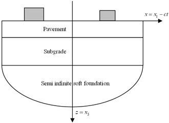
Two dimensional models are not able to reproduce mechanisms of wave propagation in the ground correctly since the loading zone represents a reduced area compared to infinite ground surface, thus excluding the hypothesis of plane deformation. This limitation has motivated researchers to obtain solutions using 3D models (see Fig. 1).

2.1. Description of the model

The calculation method uses the Fourier transform formalism for a semi-analytical solution in the wave number domain. The dynamic stiffness matrix for pavement-subgrade-soft ground system is written and accompanied by a fitted phase argument in Helmoltz functions. This provides us a fast numerical approach to the problem. Equations are written in the wave number domain as well as for steady state solutions. In this paper, the steady-state response means all the components of response are assumed to be time-harmonic form, which is consistent with dynamic loading. An inverse numerical Fourier transform is then applied when the matrix equation of the whole system (pavement-subgrade-soft ground system) has been solved.

Fig. 13D model of pavement-subgrade-soft ground system and the tandem-axle loads

(a)

(b)

2.2. Analytical solution of single-phase elastic soil

For an elastic, homogeneous and isotropic layer, the equation of motion is:

1

G_{e} u_{i, j j}^{e} + (λ_{e} + G_{e}) u_{j, j i}^{e} = ρ_{e} {\ddot{u}}_{i}^{e}

,

where $u^{e}$ is the vector of displacements for elastic soil, $ρ_{e}$ is the mass density of the solid and $G_{e}$ , $λ_{e}$ are the Lame’s constants, and for the behaviour law:

2

τ_{i j}^{e} = λ_{e} θ_{e} δ_{i j} + 2 G_{e} ε_{i j}^{e},

where $τ^{e}$ , $ε^{e}$ are the vector of stresses and strains for elastic soil, $δ_{i j}$ is the Kronecker delta, and $θ_{e}$ is the volumetric strain of the soil. To define elastic body waves ( $P$ – and $S$ – waves), Helmholtz’s potentials $ϕ$ and $ψ$ are usually used, so that:

3

u^{e} = \nabla ϕ + \nabla \land ψ

In this paper, the Fourier transforms with respect to $x$ and $y$ coordinate are defined as:

4

\bar{f} (β, λ, z, t) = \int_{- \infty}^{\infty} \int_{- \infty}^{\infty} f (x, y, z, t) e^{- i (β x + γ y)} d x d y .

The inverse relationship is given by the following form:

5

f (x, y, z, t) = \frac{1}{4 π^{2}} \int_{- \infty}^{\infty} \int_{- \infty}^{\infty} \bar{f} (β, λ, z, t) e^{i (β x + γ y)} d β d γ,

where $β$ , $γ$ are the wave number in the $x$ and $y$ direction, $f$ is a variable in space domain, and $\bar{f}$ is the corresponding variable in the transformed domain.

By using the Fourier transforms given in Eq. (4), Eqs. (1)-(3) and the solid strain equation are transformed from partial differential equations to ordinary differential equations. The typical vehicle excitation is composed of a set of vertical components that symbolize the effect of each wheel on the pavement. Each of these forces is taken as harmonic. The “fitted phase angle” is defined by Helmholtz’s potentials [7], so that:

6

\{\begin{array}{l} ϕ = A_{1} e^{α_{1} (z - h)} + A_{2} e^{- α_{2} z}, \\ ψ = A_{3} e^{α_{1} (z - h)} + A_{4} e^{- α_{2} z}, \end{array}

where $α_{i} = \sqrt{β^{2} + γ^{2} - k_{i}^{2}}$ , $i = 1, 2;$ $k_{i} = (Ω_{0} - β c) / c_{i}$ , $i = 1, 2;$ $c_{1} = \sqrt{(λ_{e} + 2 G_{e}) / ρ_{e}}$ and $c_{2} = \sqrt{G_{e} / ρ_{e}}$ are the compression ( $P$ -waves) and shear wave ( $S$ -waves) speed of single-phase elastic soil, respectively; $Ω_{0}$ is the excitation frequency, $c$ is the vehicle speed and $h$ is the thickness of the soil layer. Because of numerical difficulties due to exponential terms in the rigidity matrix, layers must be divided into several sub-layers increasing the number of iterations. In fact, the role of the fitted phase translation is to solve this problem by excluding exponential terms (growing exponential) in the dynamic stiffness matrix thus providing good condition.

A change of variables (translation in the mobile reference linked to the load) and functions (evaluation of the steady state solution) as well as the use of spatial Fourier transform lead to the calculation of displacements and stresses in the wave number domain, as in Lu [26]:

7

{\bar{u}}_{x}^{e} = \frac{- i β e^{α_{1} (z - h)}}{k_{1}^{2}} A_{1} + \frac{- i β e^{- α_{1} z}}{k_{1}^{2}} A_{2} + e^{α_{2} (z - h)} A_{3} + e^{- α_{2} z} A_{4},

8

{\bar{u}}_{y}^{e} = \frac{- i γ e^{α_{1} (z - h)}}{k_{1}^{2}} A_{1} + \frac{- i γ e^{- α_{1} z}}{k_{1}^{2}} A_{2} + e^{α_{2} (z - h)} A_{5} + e^{- α_{2} z} A_{6},

9

{\bar{u}}_{z}^{e} = \frac{- α_{1} e^{α_{1} (z - h)}}{k_{1}^{2}} A_{1} + \frac{α_{1} e^{- α_{1} z}}{k_{1}^{2}} A_{2} + \frac{- i β}{α_{2}} e^{α_{2} (z - h)} A_{3} + \frac{i β}{α_{2}} e^{- α_{2} z} A_{4} + \frac{- i γ}{α_{2}} e^{α_{2} (z - h)} A_{5} + \frac{i γ}{α_{2}} e^{- α_{2} z} A_{6},

10

{\bar{τ}}_{x z}^{e} = G_{e} [\frac{- 2 i β α_{1}}{k_{1}^{2}} e^{α_{1} (z - h)} A_{1} + \frac{2 i β α_{1}}{k_{1}^{2}} e^{- α_{1} z} A_{2} + \frac{(α_{2}^{2} + β^{2})}{α_{2}} e^{α_{2} (z - h)} A_{3} - \frac{(α_{2}^{2} + β^{2})}{α_{2}} e^{- α_{2} z} A_{4} + \frac{β γ}{α_{2}} e^{α_{2} (z - h)} A_{5} - \frac{β γ}{α_{2}} e^{- α_{2} z} A_{6}],

11

{\bar{τ}}_{y z}^{e} = G_{e} [\frac{- 2 i γ α_{1}}{k_{1}^{2}} e^{α_{1} (z - h)} A_{1} + \frac{2 i γ α_{1}}{k_{1}^{2}} e^{- α_{1} z} A_{2} + \frac{β γ}{α_{2}} e^{α_{2} (z - h)} A_{3} - \frac{β γ}{α_{2}} e^{- α_{2} z} A_{4} + \frac{(α_{2}^{2} + γ^{2})}{α_{2}} e^{α_{2} (z - h)} A_{5} - \frac{(α_{2}^{2} + γ^{2})}{α_{2}} e^{- α_{2} z} A_{6}],

12

{\bar{τ}}_{z z}^{e} = G_{e} [\frac{- (2 α_{2}^{2} + k_{2}^{2})}{k_{1}^{2}} e^{α_{1} (z - h)} A_{1} - \frac{(2 α_{2}^{2} + k_{2}^{2})}{k_{1}^{2}} e^{- α_{1} z} e^{- α_{1} z} A_{2} - 2 i β e^{α_{2} (z - h)} A_{3} - 2 i β e^{- α_{2} z} A_{4} - 2 i γ e^{α_{2} (z - h)} A_{5} - 2 i γ e^{- α_{2} z} A_{6}],

where $({\bar{u}}_{x}^{e}, {\bar{u}}_{y}^{e}, {\bar{u}}_{z}^{e})$ is the transformed displacement vector and $({\bar{τ}}_{x z}^{e}, {\bar{τ}}_{y z}^{e}, {\bar{τ}}_{z z}^{e})$ is the stress vector; $A_{1} ~ A_{6}$ are arbitrary constants.

2.3. Analytical solution of poroelastic half-space

The soft subsoil medium is modeled as a uniform poroelastic half-space, fully saturated by the viscous fluid. The fluid is free to flow throughout the upper surface of the soil. The governing equations of a fully fluid-saturated poroelastic soil, based on the assumption of incompressible solid grains and neglecting the apparent mass density, are given by Biot [16]:

13

G_{s} u_{i, j j}^{s} + (λ_{s} + α^{2} M + G_{s}) u_{j, j i}^{s} + α M w_{j, j i}^{s} = ρ {\ddot{u}}_{i}^{s} + ρ_{f} {\ddot{w}}_{i}^{s}

14

α M u_{j, j i}^{s} + M w_{j, j i}^{s} = ρ_{f} {\ddot{u}}_{i}^{s} + \frac{ρ_{f}}{n} {\ddot{w}}_{i}^{s} + \frac{η_{w}}{k_{d}} {\dot{w}}_{i}^{s}

The constitutive relationships of the saturated soil medium are given as follows:

15

τ_{i j}^{s} = λ_{s} θ_{s} δ_{i j} + 2 G_{s} ε_{i j}^{s} - δ_{i j} α p,

16

- {\dot{p}}_{s} = M {\dot{w}}_{i, i}^{s} + α M {\dot{u}}_{i, i}^{s},

where $u_{i}^{s}$ and $w_{i}^{s}$ are the displacements of the solid skeleton and the infiltration displacement of the pore fluid, respectively, in the $x$ , $y$ and $z$ directions; $G_{s}$ and $λ_{s}$ are Lame constants; $α$ and $M$ denote of the compressibility of the soil and fluid (under the assumption of incompressible solid grains, $α =$ 1, $M = K_{f} / n$ ); and $K_{f}$ is the bulk modulus of the fully saturated fluid. The parameters $η_{w}$ , $k_{d}$ represent the fluid viscosity and the intrinsic permeability of the soil medium, respectively; $ρ = n ρ_{f} + (1 - n) ρ_{s}$ , where $ρ_{f}$ and $ρ_{s}$ are the mass densities of the fluid and solid and $n$ is the porosity. $τ_{i j}^{s}$ is the total stress components of the bulk material, and $p_{s}$ is the pore water pressure.

By applying the Fourier transforms given in Eq. (4), Eqs. (13)-(16) and the solid strain equation are transformed from partial differential equations to ordinary differential equations. By resolving the ordinary differential equations, one can obtain the responses of the displacements and the stresses of the poroelastic half-space, as given by Lu [26]:

17

\begin{array}{l} {\bar{u}}_{x, s} = i β e^{- α_{3} z} A_{7} + i β e^{- α_{4} z} A_{8} + α_{5} e^{- α_{5} z} A_{10}, \\ {\bar{u}}_{y, s} = i γ e^{- α_{3} z} A_{7} + i γ e^{- α_{4} z} A_{8} - α_{5} e^{- α_{5} z} A_{9}, \\ {\bar{u}}_{z, s} = - α_{3} e^{- α_{3} z} A_{7} - α_{4} e^{- α_{4} z} A_{8} - i γ e^{- α_{5} z} A_{9} + i β e^{- α_{5} z} A_{10}, \\ {\bar{w}}_{z, s} = - α_{3} ε_{3} e^{- α_{3} z} A_{7} - α_{4} ε_{4} e^{- α_{4} z} A_{8} - i γ ε_{5} e^{- α_{5} z} A_{9} + i β ε_{5} e^{- α_{5} z} A_{10}, \end{array}

18

\begin{array}{l} {\bar{τ}}_{x z, s} = G_{s} [- 2 i β α_{3} e^{- α_{3} z} A_{7} - 2 i β α_{4} e^{- α_{4} z} A_{8} + 2 β γ e^{- α_{5} z} A_{9} - (α_{5}^{2} + β^{2}) e^{- α_{5} z} A_{10}], \\ {\bar{τ}}_{y z, s} = G_{s} [- 2 i γ α_{3} e^{- α_{3} z} A_{7} - 2 i γ α_{4} e^{- α_{4} z} A_{8} + (α_{5}^{2} + γ^{2}) e^{- α_{5} z} A_{9} - 2 β γ e^{- α_{5} z} A_{10}], \\ {\bar{τ}}_{z z, s} = G_{s} [m_{3} e^{- α_{3} z} A_{7} + m_{4} e^{- α_{4} z} A_{8} + 2 i γ α_{5} e^{- α_{5} z} A_{9} - 2 i β α_{5} e^{- α_{5} z} A_{10}], \\ {\bar{p}}_{s} = G_{s} [n_{3} e^{- α_{3} z} A_{7} + n_{4} e^{- α_{4} z} A_{8}], \end{array}

where $A_{7} ~ A_{10}$ are arbitrary constants determined by boundary conditions, other symbols in Eqs. (17) and (18) are detailed as follows:

19

α_{3,4}^{2} = β^{2} + γ^{2} - γ_{3,4}^{2} and α_{5}^{2} = β^{2} + γ^{2} - γ_{5}^{2},

20

m_{3,4} = 2 α_{3,4}^{2} - (λ_{s} + α^{2} M + α M ε_{3,4}) γ_{3,4}^{2} / G_{s} and n_{3,4} = (α + ε_{3,4}) M γ_{3,4}^{2} / G_{s},

21

ε_{3,4} = - \frac{[(λ_{s} + α^{2} M + 2 G_{s}) γ_{3,4}^{2} + ρ χ_{1}]}{ρ_{w} χ_{1} + α M γ_{3,4}^{2}} and ε_{5} = - \frac{ρ_{w} χ_{1}}{m χ_{1} + b χ_{2}},

22

γ_{3,4}^{2} = \frac{L_{2} \pm \sqrt{L_{2}^{2} - 4 L_{1} L_{3}}}{2 L_{1}} and γ_{5}^{2} = - \frac{L_{3}}{[G_{s} (m χ_{1} + b χ_{2})]},

23

\{\begin{array}{l} L_{1} = M (λ_{s} + 2 G_{s}), \\ L_{2} = 2 α M ρ_{f} χ_{1} - (λ_{s} + α^{2} M + 2 G_{s}) (m χ_{1} + b χ_{2}) - ρ χ_{1} M, \\ L_{3} = ρ χ_{1} (m χ_{1} + b χ_{2}) - ρ_{f}^{2} χ_{1}^{2}, \\ χ_{1} = - ω^{2}, \\ χ_{2} = i ω . \end{array}

It should be noted that, as $z \to \infty$ , the dynamic responses become zero; therefore, the real part of $α_{3}$ , $α_{4}$ and $α_{5}$ must be positive.

2.4. Dynamic stiffness matrix of pavement-subgrade-soft ground system

In this part, the previous model (Fig. 1) is used with two single-phase elastic layers on a poroelastic half-space. For the pavement with thickness $h_{p}$ , the displacements at the surface and bottom of the layer are written in terms of the constants $A_{1}$ , $A_{2}$ , $A_{3}$ , $A_{4}$ , $A_{5}$ and $A_{6}$ according to Eqs. (7)-(9):

24

\{{\bar{U}}_{P}\} = {\{\begin{matrix} {\bar{u}}_{x, p}^{(0)} & {\bar{u}}_{y, p}^{(0)} & i {\bar{u}}_{z, p}^{(0)} & {\bar{u}}_{x, p}^{(1)} & {\bar{u}}_{y, p}^{(1)} & i {\bar{u}}_{z, p}^{(1)} \end{matrix}\}}^{T} = [D^{p}] {\{\begin{matrix} A_{1} & A_{2} & A_{3} & A_{4} & A_{5} & A_{6} \end{matrix}\}}^{T},

where the superscripts ‘(0)’ and ‘(1)’ denote the surface and bottom of the layer, respectively. $[D^{p}]$ is displacement matrix for pavement.

Similarly, for the same layer, stresses can be expressed in terms of the previous constants:

25

\{{\sum^{¯}}_{P}\} = {\{\begin{matrix} - {\bar{τ}}_{x z, p}^{(0)} & - {\bar{τ}}_{y z, p}^{(0)} & - i {\bar{τ}}_{z z, p}^{(0)} & {\bar{τ}}_{x z, p}^{(1)} & {\bar{τ}}_{y z, p}^{(1)} & i {\bar{τ}}_{z z, p}^{(1)} \end{matrix}\}}^{T} = [S^{p}] {\{\begin{matrix} A_{1} & A_{2} & A_{3} & A_{4} & A_{5} & A_{6} \end{matrix}\}}^{T},

where $[S^{p}]$ is stress matrix for pavement.

According to Eqs. (24) and (25), a relation between displacements and stresses can be written into a matrix formulation:

26

{{\sum^{¯}}_{P}} = [S^{p}] {[D^{p}]}^{- 1} {{\bar{U}}_{P}} = [K^{p}] {{\bar{U}}_{P}},

where $[K^{p}] = [S^{p}] {[D^{p}]}^{- 1}$ is dynamic stiffness matrix for pavement.

Similarly, for the second layer of elastic medium, a relation between displacements and stresses can be written into a matrix formulation:

27

{{\sum^{¯}}_{e}} = [S^{e}] {[D^{e}]}^{- 1} {{\bar{U}}_{e}} = [K^{e}] {{\bar{U}}_{e}},

whereis $[K^{e}] = [S^{e}] {[D^{e}]}^{- 1}$ dynamic stiffness matrix for subgrade.

For the poroelastic half-space, the displacements and stresses at the surface of the half-space are written in terms of the constants $A_{7}$ , $A_{8}$ , $A_{9}$ and $A_{10}$ according to Eqs. (17)-(18):

28

\{{\bar{U}}_{s}\} = {\{\begin{matrix} {\bar{u}}_{x, s}^{(2)} & {\bar{u}}_{y, s}^{(2)} & i {\bar{u}}_{z, s}^{(2)} & {\bar{w}}_{z, s}^{(2)} \end{matrix}\}}^{T} = [D^{s}] {\{\begin{matrix} A_{7} & A_{8} & A_{9} & A_{10} \end{matrix}\}}^{T},

29

{{\sum^{¯}}_{s}} = {\begin{matrix} - {\bar{τ}}_{x z, s}^{(2)} & - {\bar{τ}}_{y z, s}^{(2)} & - i {\bar{τ}}_{z z, s}^{(2)} & - {\bar{p}}_{s}^{2} \end{matrix}} = [S^{s}] {\begin{matrix} A_{7} & A_{8} & A_{9} & A_{10} \end{matrix}}^{T},

where the superscript ‘(2)’ denotes the surface of the half-space. $[D^{s}]$ , $[S^{s}]$ are displacement matrix and stress matrix for the poroelastic half-space.

From Eqs. (28) and (29), the following relation between displacements and stresses can be derived:

30

{{\sum^{¯}}_{s}} = [S^{s}] {[D^{s}]}^{- 1} {{\bar{U}}_{s}} = [K^{s}] {{\bar{U}}_{s}},

where $[K^{s}] = [S^{s}] {[D^{s}]}^{- 1}$ is dynamic stiffness matrix for poroelastic half-space.

Assuming that the contact conditions among the layers are smooth, the displacements and the stresses are continuous at the interfaces. Thus, the following continuity conditions hold at each interface:

31

{\{\begin{matrix} {\bar{τ}}_{x z, p}^{(1)} & {\bar{τ}}_{y z, p}^{(1)} & {\bar{τ}}_{z z, p}^{(1)} & {\bar{u}}_{x, p}^{(1)} & {\bar{u}}_{y, p}^{(1)} & {\bar{u}}_{z, p}^{(1)} \end{matrix}\}}^{T} = {\{\begin{matrix} {\bar{τ}}_{x z, e}^{(1)} & {\bar{τ}}_{y z, e}^{(1)} & {\bar{τ}}_{z z, e}^{(1)} & {\bar{u}}_{x, e}^{(1)} & {\bar{u}}_{y, e}^{(1)} & {\bar{u}}_{z, e}^{(1)} \end{matrix}\}}^{T},

32

{\{\begin{matrix} {\bar{τ}}_{x z, e}^{(2)} & {\bar{τ}}_{y z, e}^{(2)} & {\bar{τ}}_{z z, e}^{(2)} & {\bar{u}}_{x, e}^{(2)} & {\bar{u}}_{y, e}^{(2)} & {\bar{u}}_{z, e}^{(2)} \end{matrix}\}}^{T} = {\{\begin{matrix} {\bar{τ}}_{x z, s}^{(2)} & {\bar{τ}}_{y z, s}^{(2)} & {\bar{τ}}_{z z, s}^{(2)} & {\bar{u}}_{x, s}^{(2)} & {\bar{u}}_{y, s}^{(2)} & {\bar{u}}_{z, s}^{(2)} \end{matrix}\}}^{T} .

As the contact surface between the subgrade and the poroelastic half-space is assumed to be fully permeable, the following expression can be derived:

33

{\bar{p}}_{s}^{2} = 0 .

From Eqs. (26)-(27) and Eqs. (30)-(33), the 3D stiffness matrix is the combination of the stiffness matrices of each layer, the following relationship is given in a matrix form as:

34

\{\begin{matrix} - {\bar{τ}}_{x z, p}^{(0)} \\ - {\bar{τ}}_{y z, p}^{(0)} \\ - i {\bar{τ}}_{z z, p}^{(0)} \\ 0 \\ 0 \\ 0 \\ 0 \\ 0 \\ \begin{matrix} 0 \\ 0 \end{matrix} \end{matrix}\} = [\begin{matrix} K_{11}^{p} & K_{12}^{p} & K_{13}^{p} & K_{14}^{p} & K_{15}^{p} & K_{16}^{p} & 0 & 0 & 0 & 0 \\ K_{21}^{p} & K_{22}^{p} & K_{23}^{p} & K_{24}^{p} & K_{25}^{p} & K_{26}^{p} & 0 & 0 & 0 & 0 \\ K_{31}^{p} & K_{32}^{p} & K_{33}^{p} & K_{34}^{p} & K_{35}^{p} & K_{36}^{p} & 0 & 0 & 0 & 0 \\ K_{41}^{p} & K_{42}^{p} & K_{43}^{p} & K_{44}^{p} + K_{11}^{e} & K_{45}^{p} + K_{12}^{e} & K_{46}^{p} + K_{13}^{e} & K_{14}^{e} & K_{15}^{e} & K_{16}^{e} & 0 \\ K_{51}^{p} & K_{52}^{p} & K_{53}^{p} & K_{54}^{p} + K_{21}^{e} & K_{55}^{p} + K_{22}^{e} & K_{56}^{p} + K_{23}^{e} & K_{24}^{e} & K_{25}^{e} & K_{26}^{e} & 0 \\ K_{61}^{p} & K_{62}^{p} & K_{63}^{p} & K_{64}^{p} + K_{31}^{e} & K_{65}^{p} + K_{32}^{e} & K_{66}^{p} + K_{33}^{e} & K_{34}^{e} & K_{35}^{e} & K_{36}^{e} & 0 \\ 0 & 0 & 0 & K_{41}^{e} & K_{42}^{e} & K_{43}^{e} & K_{44}^{e} + K_{11}^{s} & K_{45}^{e} + K_{12}^{s} & K_{46}^{e} + K_{13}^{s} & K_{14}^{s} \\ 0 & 0 & 0 & K_{51}^{e} & K_{52}^{e} & K_{53}^{e} & K_{54}^{e} + K_{21}^{s} & K_{55}^{e} + K_{22}^{s} & K_{56}^{e} + K_{23}^{s} & K_{24}^{s} \\ \begin{matrix} 0 \\ 0 \end{matrix} & \begin{matrix} 0 \\ 0 \end{matrix} & \begin{matrix} 0 \\ 0 \end{matrix} & \begin{matrix} K_{61}^{e} \\ 0 \end{matrix} & \begin{matrix} K_{62}^{e} \\ 0 \end{matrix} & \begin{matrix} K_{63}^{e} \\ 0 \end{matrix} & \begin{matrix} K_{64}^{e} + K_{31}^{s} \\ K_{41}^{s} \end{matrix} & \begin{matrix} K_{65}^{e} + K_{32}^{s} \\ K_{42}^{s} \end{matrix} & \begin{matrix} K_{66}^{e} + K_{33}^{s} \\ K_{43}^{s} \end{matrix} & \begin{matrix} K_{34}^{s} \\ K_{44}^{s} \end{matrix} \end{matrix}] \{\begin{matrix} {\bar{u}}_{x, p}^{(0)} \\ {\bar{u}}_{y, p}^{(0)} \\ i {\bar{u}}_{z, p}^{(0)} \\ {\bar{u}}_{x, p}^{(1)} \\ {\bar{u}}_{y, p}^{(1)} \\ i {\bar{u}}_{z, p}^{(1)} \\ {\bar{u}}_{x, e}^{(2)} \\ {\bar{u}}_{y, e}^{(2)} \\ \begin{matrix} i {\bar{u}}_{z, e}^{(2)} \\ {\bar{w}}_{z, s}^{(2)} \end{matrix} \end{matrix}\} .

Consequently, the displacement vector at the interface of each layer is given by:

35

{\bar{U}} = [B] {\sum^{¯}} = {[K]}^{- 1} {\sum^{¯}},

where $[B]$ is the inverse stiffness matrix whose size is 10×10 of pavement-subgrade-soft ground system.

2.5. Description of the traffic load

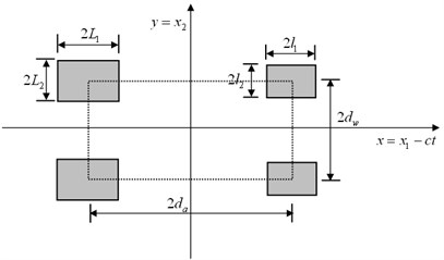
The shape of the tire-pavement contact area is assumed to be square, as shown in Fig. 1, and any change in the shape during load variation is neglected. The variations of the load amplitude resulting from the pavement surface roughness and the mechanical system of the vehicle are neglected. The traffic load is modeled as four rectangular load pressures expressed as in Eq. (36):

36

f (x_{1}, y_{1}, t) = \{\begin{array}{l} \frac{q_{0} e^{i Ω_{0} t}}{4 l_{1} l_{2}}, & (d_{a} - l_{1}) \leq x_{1} - c t \leq (d_{a} + l_{1}) and (d_{w} - l_{2}) \leq |y_{1}| \leq (d_{w} + l_{2}), \\ \frac{Q_{0} e^{i Ω_{0} t}}{4 L_{1} L_{2}}, & - (d_{a} + L_{1}) \leq x_{1} - c t \leq - (d_{a} - L_{1}) and (d_{w} - L_{2}) \leq |y_{1}| \leq (d_{w} + L_{2}), \\ 0, & otherwise, \end{array}

where $q_{0}$ and $Q_{0}$ are the magnitude of the load pressure for the front and the rear wheel, respectively. $2 l_{1}$ , $2 l_{2}$ are the loaded lengths of a tire print in the $x_{1}$ and $y_{1}$ directions, respectively, for the front wheel, and $2 L_{1}$ , $2 L_{2}$ are the loaded lengths of a tire print in the $x_{1}$ and $y_{1}$ directions, respectively, for the rear wheel. $2 d_{a}$ is the distance between the front and rear wheels, and $2 d_{w}$ is the distance between the left and right wheels.

A change of variables (translation in the mobile reference linked to the load) and functions (evaluation of the steady state solution) as well as the use of spatial Fourier transform lead to the expression of traffic load in the wave number domain:

37

\bar{f} (β, γ, t) = \bar{f} (β, γ) \cdot e^{i Ω_{0} t} = [\frac{q_{0} s i n (β l_{1}) s i n (γ l_{2})}{β γ l_{1} l_{2}} e^{- i β d_{a}} + \frac{Q_{0} s i n (β L_{1}) s i n (γ L_{2})}{β γ L_{1} L_{2}} e^{i β d_{a}}] (e^{- i γ d_{w}} + e^{i γ d_{w}}) \cdot e^{i Ω_{0} t} .

As no lateral and longitudinal stress is considered in the present problem, the following boundary conditions, omitting the common time factor, $e^{{i Ω}_{0} t}$ , can be obtained at the surface of pavement:

38

{\bar{τ}}_{y z, p}^{(0)} = {\bar{τ}}_{z z, p}^{(0)} = 0, {\bar{τ}}_{z z, p}^{(0)} = - \bar{f} (β, γ) .

Substituting Eqs. (37) and (38) into Eq. (35), the displacements in the transformed domain can be obtained as follows:

39

{\bar{U}} = [B] {\sum^{¯}} = [B] {[\begin{matrix} 0 & 0 & i \bar{f} (β, γ) & 0 & 0 & 0 & 0 & 0 & 0 & 0 \end{matrix}]}^{T} .

After the displacements at the interface of layers are determined, it is rather straightforward to obtain all the stresses at an arbitrary interface. Furthermore, the constants of each layer can be determined, and the stresses and displacements in an arbitrary depth of the road structures can also be derived.

Once the transformed stress and displacement components are determined, the actual medium response can be established by means of the Fourier inversion theorem from Eq. (5). It should be noted that all the exponential functions involved in the present formulation contain only non-positive exponents, which are critical for numerical stability. Taking the surface of half-space for example, the displacements in the time domain can be expressed as follows:

40

\{\begin{matrix} u_{x, e}^{(2)} \\ u_{y, e}^{(2)} \\ i u_{z, e}^{(2)} \end{matrix}\} = \frac{1}{4 π^{2}} \int_{- \infty}^{\infty} \int_{- \infty}^{\infty} \{\begin{matrix} B_{73} \\ B_{83} \\ B_{93} \end{matrix}\} i \bar{f} (β, γ) \cdot e^{i (β x + γ y)} \cdot e^{i Ω_{0} t} d β d γ .

2.6. Comparison with existing work

To compute the inverse transform accurately with a discrete transform, the mesh of the calculated functions must be fine enough to accurately represent the details of the functions, and the integrals must be truncated at values high enough to avoid distorting the results. To satisfy the above requirements, a FFT algorithm is employed with a grid of 2048×2048 points with ranges of 16 m^-1 $< β <$ 16 m^-1 and 16 m^-1 $< γ <$ 16 m^-1 is adopted.

Table 1Parameters for fully water-saturated poroelastic soil medium [27]

Lame constant $λ_{s} / \times 10^{7} P a$	1.0
Lame constant $G_{s} / \times 10^{7} P a$	3.0
Solid density $ρ_{s} /$ (g/cm³)	2.5
Compress-wave velocity $c_{S S} /$ (m/s)	140
Shear-wave velocity $c_{S H} /$ (m/s)	121
Porosity $n$	0.3
Compressibility parameter $α$	0.95
Compressibility parameter $M / \times 10^{9} P a$	5.0
Ratio between fluid viscosity and the permeability $b / (10^{10} m^{- 1} s)$	1.0
Water density $ρ_{w} /$ (g/cm³)	1.0

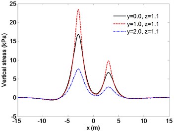
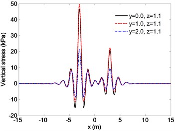
To verify the accuracy of this work, Fig. 2 compares the vertical stresses and displacements obtained from our model with that given by Lu et al. [27]. Their work studied the three-dimensional steady-state response of a poroelastic half-space soil medium subjected to a moving point load. By selecting the parameters of pavement and subgrade ( $E_{p} = E_{e} =$ 0, $h_{p} = h_{e} =$ 0) and the same parameters of the soil medium (as shown in Table. 1) and load as those in Lu et al. [27], one can calculate the stresses and displacements. Then, the stresses and displacements are non-dimensionalized as $σ_{z z}^{*} = σ_{z z} a_{R}^{2} / T$ and $u_{i}^{*} = (u_{i} G_{R} \cdot a_{R}) / T$ $(i = x, y, z)$ , respectively, and the coordinates are non-dimensionalized as $x^{*} = x / a_{R}$ , $y^{*} = y / a_{R}$ , $z^{*} = z / a_{R}$ , where $a_{R} =$ 1 m, is the reference length; $G_{R} =$ 3.0×10⁹ Pa, is the reference shear modulus; $c_{S H}$ is the shear-wave velocity which is defined as $c_{S H} = \sqrt{G_{s} / ρ}$ , and $T$ is the load pressure. The dynamic responses of the observation with coordinates $y = z =$ 1.0 are calculated in Fig. 2. The agreement between the two solutions, as far as the vertical stress and displacement is concerned, is excellent.

Fig. 2Comparison between present work and Lu et al.’s [27] work

(a) Vertical stress

(b) Vertical displacement

3. Numerical results and discussion

In order to investigate the response characteristics of the pavement-subgrade-soft ground system, Saga airport road [28] is selected and analyzed by the proposed method. Saga airport road was constructed from 1990 to 1992 with a total length of 9 km. At the site, there is about 20-m-thick highly compressible and highly sensitive Ariake clay. The typical cross section of Saga airport road is composed of three layers: asphalt surface layer, subgrade with decomposed granite and soft subsoil with Ariake clay. The physical and mechanical properties of the road structure layers are given in Table 2, and they correspond to those given in Chai [28], and the parameters of the tandem-axle loads are given in Table 3, corresponding to the heavy truck adopted by Chai [28]. The main physical quantities of interest in this investigation are the vertical displacements, stresses, and accelerations of the soft subsoil. The variations of these quantities with respect to the coordinates, the load velocity and frequency, the thickness and the modulus of the sugrade, and the permeability coefficient of the soft subsoil are studied.

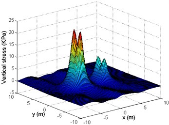
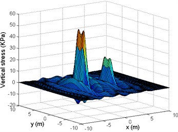
In Fig. 3, the vertical stresses of the points with coordinates – $15 m \leq x \leq 15 m$ , $z = 1.1 m$ and $y =$ 0.0 m, 1.0 m, 2.0 m, respectively, are calculated for two kinds of load velocities, $c = 0.1 c_{s s}$ and $c = 0.9 c_{s s}$ , where $c_{s s}$ is the shear wave velocity of the saturated poroelastic half-space. It can be seen from Fig. 3(a) that, when $c = 0.1 c_{ss}$ , two stress peaks appear at the points where the load is applied. The values of the peaks for rear wheel are larger than that for front wheel, and this is because the rear-axle weight of the heavy trucks is larger than front-axle weight. In terms of different points $y =$ 0.0 m, 1.0 m, 2.0 m, the stress for $y =$ 1.0 m is the largest, and the stress for $y =$ 0.0 m is larger than that for $y =$ 2.0 m, which indicates that the maximum response occurs beneath the point where the load is applied. When $c = 0.9 c_{s s}$ , as shown in Fig. 3(b), the magnitude of the stresses is much larger than that in Fig. 3(a), and significant ground vibration is observed, which is obviously due to the fact that velocity $0.9 c_{s s}$ is very close to the Rayleigh wave velocity of the porous medium. The vertical stresses for different points $y =$ 0.0 m, 1.0 m, 2.0 m, are also presented in Fig. 3(b). The stress for $y =$ 1.0 m is the largest, which is the same of the low-load-velocity condition. In order to observe the response more clearly, the vertical stresses for two kinds of load velocities, $c = 0.1 c_{s s}$ and $c = 0.9 c_{s s}$ are calculated in plane – $10 m \leq x \leq 10 m$ , – $10 m \leq y \leq 10 m$ , as shown in Fig. 4. It is clear in Fig. 4 that four peaks can be observed in the plane, which corresponds to four wheels of the vehicle. The magnitude of the stresses for the high velocity of $c = 0.9 c_{s s}$ is much larger than that for the low velocity of $c = 0.1 c_{s s}$ , and the stresses apparently vibrate to a wide extent.

Table 2Physical and mechanical properties of each layer (Saga Airport Road)

Layers	Asphalt concrete	Subgrade	Soft subsoil
Thickness / m	0.1	1.0	–
Elastic modulus $E$ / MPa	1000	35	10
Poisson’s ratio $ν$	0.3	0.35	0.4
Solid density $ρ_{s}$ / kg m^-3	–	–	1700
Water density $ρ_{f}$ / kg m^-3	–	–	1000
Soil density $ρ$ / kg m^-3	2200	2000	1490
Porosity $n$	–	–	0.3
Compressibility parameter $α$	–	–	0.95
Compressibility parameter $M$ / MPa	–	–	5.0×10⁹
Fluid viscosity $η$	–	–	0.1
Intrinsic permeability $k$ / (m³s/kg)	–	–	1.0×10^-11

Table 3Parameters of tandem axle loads for heavy truck

Weight of front wheel $q_{0}$ (kN)	30
Weight of rear wheel $Q_{0}$ (kN)	70
Loaded length of front wheel $2 l_{1}$ (m)	0.32
Loaded width of front wheel $2 l_{2}$ (m)	0.32
Loaded length of rear wheel $2 L_{1}$ (m)	0.44
Loaded width of rear wheel $2 L_{2}$ (m)	0.44
Distance between front and rear wheels $2 d_{a}$ (m)	6
Distance between right and left wheels $2 d_{w}$ (m)	2

Fig. 3Distribution of the vertical stresses for different observation points

(a) $c = 0.1 c_{s s}$

(b) $c = 0.9 c_{s s}$

Fig. 4Distribution of the vertical stresses in (x,y) plane

(a) $c = 0.1 c_{s s}$

(b) $c = 0.9 c_{s s}$

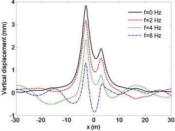
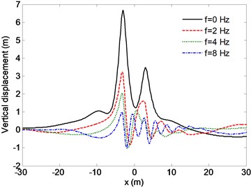
Fig. 5 shows the vertical displacements for different load excitation frequency, where $f =$ 0 Hz, $f =$ 2 Hz, $f = 4$ Hz and $f =$ 8 Hz are considered. For the sake of comparison, the displacements are presented for $z =$ 1.1 m. In Fig. 5(a), for $c = 0.1 c_{s s}$ , the displacements responses decrease as load excitation frequency increases. Two peaks appear where the load is applied when $f =$ 0 Hz and $f =$ 2 Hz, but, as load excitation frequency increases to $4$ Hz or more, a negative peak is observed near the center of the tandem axle. As the load velocity is close to the Rayleigh wave speed, as shown in Fig. 5(b), the magnitude of the displacements is much larger than that in Fig. 5(a), and the displacements response decreases rapidly with increasing load frequency. The displacements fluctuate before the load reaches the observation point.

Fig. 5Distribution of the vertical displacements for different excitation frequency

(a) $c = 0.1 c_{s s}$

(b) $c = 0.9 c_{s s}$

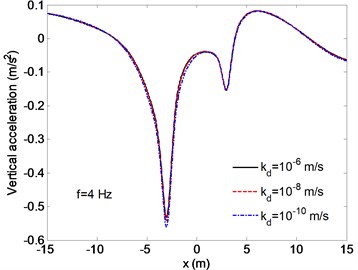
The variations of the vertical accelerations with distance $y$ for the road system at $z =$ 1.1 m are investigated in Fig. 6, where $f =$ 0 Hz, $f =$ 4 Hz and $f =$ 8 Hz are considered. It is obvious that the vertical accelerations increase rapidly with increasing load frequency. For a low load velocity of $c = 0.1 c_{s s}$ , the acceleration has two peaks at the point where the load is applied when $f =$ 0 Hz and $f =$ 4 Hz. As load excitation frequency increases to $f =$ 8 Hz, a negative peak stress is caused near the center of the tandem axle. In Fig. 6(b), the vertical accelerations for high load velocity $c = 0.9 c_{s s}$ is presented. The vertical accelerations of the soft subsoil fluctuate significantly in front of the load, and the magnitude of the vertical accelerations increases with increasing load frequency. A closer inspection of Fig. 6(b) reveals that the frequency of the acceleration fluctuations in front of the loads becomes larger as load frequency increases. Fig. 7 shows the vertical accelerations in plane – $10 m \leq x \leq 10 m$ , – $10 m \leq y \leq 10 m$ for load excitation frequency $f =$ 4 Hz. When $c = 0.1 c_{s s}$ , as shown in Fig. 7(a), the peak value of the vertical acceleration occurs where the load is applied, and no positive acceleration is caused. For the high load-velocity condition, the magnitude of the vertical acceleration is significantly larger than that for $c = 0.1 c_{s s}$ . The positive peak stresses occur near the center of the tandem axle, and the vertical acceleration fluctuates in the area in front of the load.

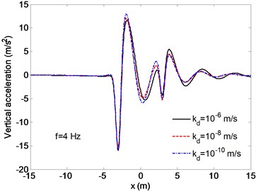
Fig. 8 presents the variations of the vertical accelerations with distance $x$ for different permeable coefficients when $f =$ 4 Hz, where $k_{d} = 10^{-6} m/s$ , $k_{d} = 10^{- 8} m/s$ and $k_{d} = 10^{- 10} m/s$ are considered. From Fig. 8(a), it can be seen that the acceleration has two peaks at the point where the load is applied. The permeability of the subsoil has little effect on soil acceleration. When the load velocity is close to the Rayleigh wave speed, as shown in Fig. 8(b), the accelerations apparently vibrate to a wide extent, the positive acceleration peak appears near the center of the tandem axle and the magnitude of the accelerations is much larger than that for the low load-velocity condition. The permeability affects the acceleration response slightly when the velocity is close to the critical speed. It also can be seen from Fig. 8 that the effect of the permeability of the soft subsoil on the magnitude of the vertical accelerations at the half-space surface is not pronounced.

Fig. 6Distribution of the vertical accelerations for different excitation frequency

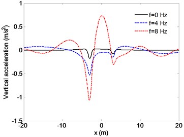
(a) $c = 0.1 c_{s s}$

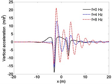
(b) $c = 0.9 c_{s s}$

Fig. 7Distribution of the vertical accelerations in (x,y) plane

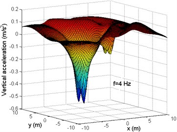
(a) $c = 0.1 c_{s s}$

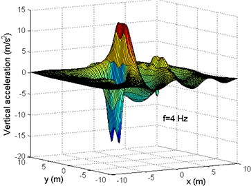
(b) $c = 0.9 c_{s s}$

Fig. 8Distribution of the vertical accelerations for different permeable coefficients

(a) $c = 0.1 c_{s s}$

(b) $c = 0.9 c_{s s}$

The effects of the properties of the road structure layers on its mechanical response are important in the design and maintenance of the road infrastructure. Therefore, further investigation of the dynamic response of road systems with different material properties is needed. In this section, the vertical stresses of different subgrade heights and Young’s modulus, which represent subgrade rigidity, are discussed. The observation point is located at the surface of the soft subsoil with coordinate – $15 m \leq x \leq 15 m$ and $y =$ 1 m, as shown in Fig. 1. In this section, the load velocity is $0.1 c_{s s}$ and frequency is 4 Hz.

In Fig. 9, the calculation parameters of the road structure layers are fixed and shown in Table 2, where the height and modulus of the subgrade varied from 1.0 to 3.0 m, and from 15 to 60 MPa, respectively. It can be seen from Fig. 9(a) that the magnitude of the vertical stresses increased sharply at the wheel action point and then gradually decreased to zero far from the wheel action point. As the subgrade height increases, the vertical stress clearly decreases, and the variations of the maximum vertical stress at different subgrade height are extremely important near the loading area but less so far from this zone. The effect of subgrade modulus on the vertical stress is presented in Fig. 9(b). The magnitude of the vertical stress decreases apparently when subgrade modulus increases from 15 to 30 MPa, but, as subgrade modulus reaches 45 MPa or more, the effect of subgrade modulus on the vertical stress is not pronounced.

Fig. 9Effect of the subgrade rigidity on the vertical stress (c=0.1css)

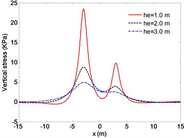
(a) Effect of the subgrade height on the stress

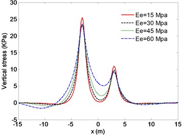
(b) Effect of the subgrade modulus on the stress

The influence of the subgrade height and Young’s modulus on the vertical stress and acceleration is further investigated, as shown in Fig. 10. In this figure the vertical stress ratio and the vertical acceleration ratio are presented as follows:

41

Vertical stresses ratio (%) =

\frac{Vertical stresses for different subgrade heights and modulus}{Vertical stresses for fixed subgrade height and {modulus (h}_{e} = 1.0 m {, E}_{e} = 10 MPa)},

42

Vertical accelerations ratio (%) =

\frac{Vertical accelerations for different subgrade heights and modulus}{Vertical accelerations for fixed subgrade height and {m o d u l u s (h}_{e} = 1.0 m {, E}_{e} = 10 MPa)} .

Fig. 10Effect of the subgrade rigidity on the response components (c=0.1css)

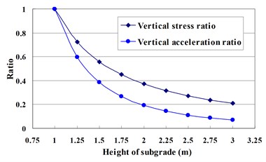
(a) Effect of the subgrade height on the responses

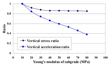
(b) Effect of the subgrade modulus on the responses

Fig. 10(a) shows that for a fixed subgrade modulus of 10 MPa and for the subgrade height varying from 1.0 to 3.0 m, the dynamic responses are sensitive to the variation in subgrade height. As the subgrade height increases, the vertical stress ratio and acceleration ratio decrease at small subgrade heights and gradually become constant at larger subgrade heights. This result explains why this factor is so important in the design of subgrade. It suggests disastrous effects on the subgrade in the case of an under-estimated height and predicts inefficiency in the case of an over-estimated height. Finally, in Fig. 10(b), the height of the subgrade is fixed at 1.0 m and its Young’s modulus varies from 10 to 80 MPa. For low subgrade modulus, the vertical stress ratio decreases until the trend become constant as a larger modulus, and the vertical acceleration ratio trends become linear with the increasing subgrade modulus. This result implies that a reasonable subgrade modulus should be chosen in the design of road.

4. Conclusions

In this paper, the steady-state response of a pavement-subgrade-soft ground system subjected to moving traffic load is studied using a semi-analytical approach. The pavement and the subgrade are regarded as two elastic layers resting on a poroelastic half-space soil medium. Four rectangular loads with a constant magnitude are used to represent the traffic load. Elastic dynamic theory for the single-phase elastic soil and Biot’s fully dynamic poroelastic theory for the saturated half-space are used to account for the model of three-layer road structure. Using the double Fourier transform, the governing equations of motion in the frequency wave-number domain are analytically solved. The fitted phase angle is employed to exclude the growing exponential terms in the dynamic stiffness matrix, which are critical for numerical stability. The expressions of the vertical stress, displacement, and acceleration in the time domain are evaluated by the inverse fast Fourier transform. The main conclusions of this study can be summarized as follows:

1. The responses in the condition of high velocity shows obvious difference from those of low velocity case, which proves that the influence of moving speed on the dynamic responses of the road system is significant.

2. The distributions of the stress, displacement, and acceleration of the soft subsoil are different for various values of loading frequency. For small values of frequency, the maximum responses occur at the point where the load is applied. As frequency increases, the positive response peaks appear and the maximum responses occur near the center of the tandem axle.

3. The acceleration has two peaks at the point where the load is applied, and the permeability of the subsoil has little effect on soil acceleration when the velocity is low. When the load velocity is close to the Rayleigh wave speed, the acceleration is much larger than that for the low load-velocity condition and apparently vibrates to a wide extent. Generally speaking, the effect of the permeability of the soft subsoil on the magnitude of the vertical accelerations at the half-space surface is not pronounced.

4. The dynamic responses of the road structure layers are sensitive to the variations in the subgrade height and Young’s modulus. The numerical calculations shows that these two parameters are extremely important in the design of subgrade and suggests potentially disastrous effects on the subgrade in the case of an under-estimated height and suggests inefficiency in the case of an over-estimated height.

References

Kausel E., Roesset J. M. Stiffness matrices for layered soil. Bulletin of the Seismological Society of America, Vol. 71, Issue 6, 1981, p. 1743-1761.

Search CrossRef
Kausel E., Peek R. Dynamic loads in the interior of a layered stratum: an explicit solution. Bulletin of the Seismological Society of America, Vol. 72, Issue 5, 1982, p. 1459-1481.

Search CrossRef
Chow Y. K., Swaddiwudhipong S., Lim S. A. Dynamic finite strip analysis of surface foundations. Earthquake Engineering and Structural Dynamics, Vol. 16, Issue 3, 1988, p. 457-467.

Search CrossRef
De Barros F. C. P., Luco J. E. Response of a layered visco-elastic half space to a moving point load. Wave Motion, Vol. 19, 1994, p. 189-210.

Search CrossRef
De Barros F. C. P., Luco J. E. Stresses and displacements in a layered half space for a moving line load. Applied Mathematics and Computation, Vol. 67, 1995, p. 103-134.

Search CrossRef
Gunaratine M., Sanders O. Response of a layered elastic medium to a moving strip load. International Journal for Numerical and Analytical Methods in Geomechanics, Vol. 20, 1996, p. 191-208.

Search CrossRef
Auersh L. Wave propagation in layered soils: theoretical solution in wave number domain and experimental results of hammer and railway traffic excitation. Journal of Sound and Vibration, Vol. 173, Issue 2, 1994, p. 233-264.

Search CrossRef
Picoux B., Rotinatb R., Regoina J. R., Houedec D. L. Prediction and measurements of vibrations from a railway track lying on a peaty ground. Journal of Sound and Vibration, Vol. 267, Issue 3, 2003, p. 575-589.

Search CrossRef
Picoux B., Houedec D. L. Diagnosis and prediction of vibration from railway trains. Soil Dynamics and Earthquake Engineering, Vol. 25, 2005, p. 905-921.

Search CrossRef
Jones D. V., Petyt M. Ground vibration in the vicinity of a rectangular load on a half space. Journal of Sound and Vibration, Vol. 166, Issue 1, 1993, p. 141-159.

Search CrossRef
Jones D. V., Petyt M. Ground vibration in the vicinity of a strip load: an elastic layer on an elastic half space. Journal of Sound and Vibration, Vol. 161, Issue 1, 1993, p. 1-18.

Search CrossRef
Jones D. V., Petyt M. Ground vibration in the vicinity of a strip load: an elastic layer on a rigid foundation. Journal of Sound and Vibration, Vol. 152, Issue 3, 1992, p. 501-515.

Search CrossRef
Skvireckas R., Kersys A., Kersys R., Lukosevicius V. Research of lateral vibrations of a passenger wagon running along the curved path. Journal of Vibroengineering, Vol. 14, Issue 2, 2012, p. 706-714.

Search CrossRef
Lu Z., Yao H. L. Effects of the dynamic vehicle-road interaction on the pavement vibration due to road traffic. Journal of Vibroengineering, Vol. 15, Issue 3, 2013, p. 1291-1301.

Search CrossRef
Biot M. A. Theory of propagation of elastic waves in a fluid-saturated porous solid. 1. Low-frequency range. Journal of the Acoustical Society of America, Vol. 28, 1956, p. 168-178.

Search CrossRef
Biot M. A. Mechanics of deformation and acoustic propagation in porous media. Journal of Applied Physics, Vol. 33, 1962, p. 1482-1498.

Search CrossRef
Theodorakopoulos D. D. Dynamic analysis of a poroelastic half-space soil medium under moving loads. Soil Dynamics and Earthquake Engineering, Vol. 23, 2003, p. 521-533.

Search CrossRef
Theodorakopoulos D. D., Chassiakoos A. P. Dynamic effects of moving load on poroelastic soil medium by an approximate method. International Journal of Solids and Structures, Vol. 256, 2004, p. 1801-1822.

Search CrossRef
Jin B. Dynamic response of a poroelastic half-space generated by high speed load. China Quarter of Mechanics, Vol. 25, 2004, p. 168-174.

Search CrossRef
Zeng X., Rajapakse R. Vertical vibrations of a rigid disk embedded in a poroelastic medium. International Journal for Numerical and Analytical Methods in Geomechanics, Vol. 23, 1999, p. 2075-2095.

Search CrossRef
Jin B. The vertical vibration of an elastic circular plate on a fluid-saturated poros half space. International Journal of Engineering Science, Vol. 37, 1999, p. 379-393.

Search CrossRef
Senjuntichai T., Sapsathiarn Y. Forced vertical vibration of circular plate in multilayered poroelastic medium. Journal of Engineering Mechanics, Vol. 129, 2003, p. 1330-1341.

Search CrossRef
Cai Y., Cao Z., Sun H. Dynamic response of pavements on poroelastic half-space soil medium to a moving traffic load. Computers and Geotechnics, Vol. 36, 2009, p. 52-60.

Search CrossRef
Lefeuve-Mesgouez G., Mesgouez A. Ground vibration due to a high-speed moving harmonic rectangular load on a poroviscoelastic half-space. International Journal of Solids and Structures, Vol. 45, Issue 11, 2008, p. 3353–3374.

Search CrossRef
Lefeuve-Mesgouez G., Mesgouez A. Three-dimensional dynamic response of a porous multilayered ground under moving loads of various distributions. Advanced Engineering Software, Vol. 46, 2012, p. 75-84.

Search CrossRef
Lu Z., Yao H. L., Cheng P. Ground vibration of soft subgrade subjected to a non-uniformly distributed train load. Rock and Soil Mechanics, Vol. 31, Issue 10, 2010, p. 3286-3294.

Search CrossRef
Lu J. F., Jeng D. S. A half-space saturated poro-elastic medium subjected to a moving point load. International Journal of Solids and Structures, Vol. 44, Issue 26, 2007, p. 573-586.

Search CrossRef
Chai J. C., Miura N. Traffic-load-induced permanent deformation of road on soft subsoil. Journal of Geotechnical and Geoenvironmental Engineering, Vol. 128, Issue 11, 2002, p. 907-916.

Search CrossRef

About this article

Received

11 September 2013

Accepted

05 October 2013

Published

15 February 2014

Keywords

FFT algorithm

moving load

pavement

soft subsoil

dynamic stiffness matrix

dynamic response

Acknowledgements

The authors gratefully acknowledge the financial support of the National 973 Project of China (No. 2013CB036405) and the Natural Science Foundation of China (No. 51209201 and 51279198).

This is an open access article distributed under the Creative Commons Attribution License, which permits unrestricted use, distribution, and reproduction in any medium, provided the original work is properly cited.