Design and validation of a railway inspection system to detect lateral track geometry defects based on axle-box accelerations registered from in-service trains

Real, T.; Montrós, J.; Montalbán, L.; Zamorano, C.; Real, J. I.

Journal of Vibroengineering

Browse Journal

Submit article

Published: 15 February 2014

Check for updates

Design and validation of a railway inspection system to detect lateral track geometry defects based on axle-box accelerations registered from in-service trains

T. Real¹

J. Montrós²

L. Montalbán³

C. Zamorano⁴

J. I. Real⁵

^{1, 2, 3, 5}Department of Transportation Engineering and Infrastructures, School of Civil Engineering Technical University of Valencia, 14 Camino de Vera, 46022 Valencia, Spain

⁴Foundation for the Research and Engineering in Railways, 160 Serrano, 28002 Madrid, Spain

Corresponding Author:

T. Real

Cite the article Download PDF

Downloads 1213

WoS Core Citations 6

Abstract

Metropolitan railway transport has become an efficient solution to the mobility necessities in urban areas. Railway track maintenance tasks have to be improved and adjusted to metropolitan requirements, in particular the few hours available to operate due to the high frequency service offered. This paper describes and proposes an inertial monitoring system to detect and estimate track irregularities by using in-service vehicles. A new maintenance strategy is established, based on the railway track conditions and continuous monitoring is provided to do so. The system proposed consists of at least two accelerometers mounted on the bogie axle-box and a GPS (Global Positioning System). Lateral accelerations have been analyzed to study gauge and lateral alignment deviations. Accelerations have been treated and processed by high-pass filtering and validation has been carried out by comparison with measurements provided by a track monitoring trolley. Measurements were made on Line 1 of the Alicante metropolitan and tram network (Spain).

1. Introduction

Mobility on medium and large cities has been one of the main issues to deal with in the last decades in order to keep a high quality transportation offer to users whereas economic, environmental and social aspects should be considered as well. Urban and metropolitan railway systems have emerged as an efficient answer to this dilemma because they do not emit poisonous gasses, they are social accepted, their cost is relatively affordable and they provide a high frequency service, suitable in medium and large cities. Demand on this kind of services is growing and thus requirements and standards must be ensured even more accurately.

Urban trains operate at high frequency and they do it during almost the whole day (up to 20 hours per day), consequently maintenance and monitoring scheduling tasks are highly limited. Regarding to maintenance scheduling optimization Zhang et al. [1] developed an enhanced genetic algorithm to search for a solution producing that the overall maintenance cost is minimized in a finite planning horizon. Predictive maintenance [2] seems to be the most efficient strategy to monitor and control track irregularities. To achieve that predictive maintenance, which is based on continuous monitoring, the utilization of in-service vehicles is required.

Traditionally the monitoring systems that were most commonly used were based on contact methods [3]. One of the main drawbacks of these systems is that, because of its own nature, they require a continuous contact with the rail. This results in a continuous wear of the rail and the monitoring system itself, so measurements are limited. In addition, contact monitoring systems reach velocities not higher than 150 km/h, because dynamic inertia affects harmfully in the contact between the contact system and the rail. Consequently non contact systems started to be developed in order to solve this inconveniences.

One of the most developed techniques is the optical based monitoring. This technique provides accurate results efficiently, nevertheless they present important handicaps: laser sensors are too expensive and they are very fragile and therefore not appropriated to work in the railway harsh conditions. Furthermore the measuring principle that optical systems employ is based in the mid-chord theory. This theory has been studied in detail by Nagamuna et al. [4], Yazawa and Takeshita [5] and Ahmadian [6]. The main conclusion taken is that this theory presents the inconvenience of filtering some wavelength defects so they cannot be detected and therefore some interesting data are neglected. Wavelet decomposition has been also studied as an alternative by Toliyat et al. [7] and Caprioli et al. [8] but more focused on rail defects than railway track ones.

Then a new monitoring system was necessary in order to avoid all these inconveniences. The inertial measuring method was developed as a non-contact alternative to the optical methods. It is based on the study of railway track starting from the register of the accelerations that the vehicle experiments throughout the track; the researches made by Kozek [9], Coudert et al. [10] and Weston et al. [11] and [12] supported this method.

As a geometrical comparison between the real state of the track and the monitored status has to be made, geometrical data are needed. Therefore accelerations are double integrated so displacements are obtained. Afterwards data has to be processed to study irregularities in the frequency domain as the standards indicate. The main and very important advantage of this system is that they can be installed on in-service railway vehicles. Then scheduled maintenance operations are simplified because interruptions on the regular service will be minimized and consequently maintenance scheduling will be optimized.

The purpose of this article is to design and validate an inertial system to obtain lateral deviations from the theoretical track geometry (gauge and alignment) from axle-box measured accelerations of an in-service train. Accelerations registered have been processed and final data have been compared with the monitoring trolley register. Measurements have been obtained on line 1 of Alicante TRAM.

2. Literature review

Regarding the inertial monitoring system several different researches have been developed so far. Many of them are focused on the utilization of non-commercial vehicles to record necessary data and others are more oriented on the advantages that the utilization of in-service vehicles offers. The choice of the different kind of accelerometers, the position where they should be installed, or the data treatment process are some of the other variables that differ from one study to another.

In the ‘90s several researches were made in the inspection and monitoring of railway track field by using specific inspection cars. Takeshita [13] and Nagamuna [14] among others started to investigate about that using the asymmetrical chord offset method. A. Carr et al. [15] did a complete study about autonomous track inspection systems, and they compiled a lot of information about the evolution of track inspection systems.

At the end of the ‘90s and during the last decade the idea of implementing the monitoring and inspection task to the current transportation vehicles appeared as a great manner to reduce costs, service cuts and therefore offer a more reliable service and increase its quality.

To relate track irregularities according to their wavelength was an interesting idea that started in 1996 and was carried out by Grassie et al. [16]. In this way frequency analysis started to be seen as an efficient manner to study track irregularities. Coudert et al. [10] employed in 1999 axle-box accelerations recordings to study railway track irregularities. They also compared two different methods for obtaining the rail profile: a conventional filtering process by means of a band-pass filter and a wavelet analysis.

In 2001 Kawasaki [17] studied track irregularities using in-service vehicles getting deep in the theoretical study of the phenomena. Accelerations where measured on the vehicle floor so many uncertainties appear such as mass and speed variations or the lateral non-linear phenomena of the movement.

As mentioned before, Yazawa and Takeshita [5] in 2002, employed the mid-chord offset method in order to correct the distortion of the waveform produced after the double integration of the accelerations. They proposed a filtering process to solve that, by using a high-pass filter, so as low frequencies will not be analyzed. The inconvenience is that they proposed the utilization of laser scanners, therefore increasing costs.

In 2007 Boccione et al. [18] investigated about the evaluation of short pitch corrugation employing axle-box mounted accelerometers on standard operating bogies. Their research is quite depth in terms of experimental data acquisition but nothing is developed about the signal processing and neither any theoretical analysis is carried out neither. Another research was made in 2010 focused on an experimental campaign test by Mannara et al. [19]. In the same year also, Weston et al. [11] and [12] accomplished a wide and complete research that had into account the experimental set-up of the procedure and the data processing made afterwards. Their research was based on measurements made by axle-box accelerometers and a bogie-mounted pitchrate gyroscope. The data processing included a double integration of the accelerations and a high-pass filter with zero phase shifts.

Other study, made in 2010 by Tsunashima et al. [20] improved the railway track monitoring by using in-service vehicles. They combined accelerometers with a GPS system to locate defects on track. Measurements are made for both conventional and high speed railway vehicles. Accelerations were measured on bogie.

This paper continues with the research started with the development of data manipulation process. Real et al. [21] started in 2010 a vehicle model and equations of motion were solved in the frequency domain. At first all the analysis was oriented to vertical alignment irregularities. In 2012, Real et al. [22] again continued improving their results by the design of an inertial set-up to measure acceleration of in-service vehicles. Comparison between inertial methods and traditional methods as monitoring trolley was made. This paper starts with the same field measurement register but it is focused on the lateral irregularities, such as gauge and lateral alignment.

3. Methodology

The procedure followed can be described into three main steps: first, data acquisition set-up has to be explained. Two data measurement campaigns were carried out: one with the inertial method proposed and another by the track monitoring trolley; necessary to validate the proposed one. Equipment, devices and the track characteristics are provided. The second step is to provide a mathematical treatment capable to process data obtained by both methods and make them comparable. Graphical and statistical comparisons were made with the two registers to validate the proposed inertial monitoring system. The last step is track monitoring itself; employing the validated inertial system and therefore defects were located and measured on track.

As mentioned before, this research follows the studies made by Real et al. [21] and [22], where vertical track defects were analyzed. In this paper lateral irregularities are studied. To do so, Spanish standards have been employed.

4. Data acquisition set-up

In order to validate the proposed inertial monitoring system is necessary to make two different inspections of the railway track. First the inertial monitoring system measurement campaign was made. Accelerometers were installed on the axle-box of the front bogie and a GPS was placed on the driver’s cabin. A regular service in the line was used to do the monitoring tasks, so no interruptions on the service were necessary. Secondly, the monitoring trolley measured a certain stretch of the track, requiring for that a service stop in the line.

Data of both registrations comes from Line 1 of Alicante TRAM, specifically from the stretch between the Mileposts 37+642 and 40+038, corresponding to Hospital Vila and Hiper Finestrat stations. It is important to remark that this stretch is limited by the track monitoring trolley, because the inertial method provides information of the whole Line 1 of the Alicante tram network as it operates with the same range as the service vehicle. This can be seen also as another advantage of the in-service vehicles over the ones based on special measurement devices as the trolley employed in this research.

4.1. Inertial monitoring system

The inertial monitoring system proposed consists of four accelerometers that have been installed on the lead bogie axle-boxes of the railway vehicle. The selected accelerometers are piezoelectric, so they will register an electrical signal after experience the vibrations of the vehicle due to the dynamic interaction with the railway track. The accelerometers selected were in particular PCB 354C02. They operate with a sensitivity of 10 mV/g and register accelerations in the three main directions $(X, Y, Z)$ on a frequency range that goes from 0.5 Hz to 20 kHz. The installation of the accelerometers has been made by means of magnetic bases fixed to the bogie in order to avoid surface drilling.

Fig. 1Accelerometer employed PCB 354 C02

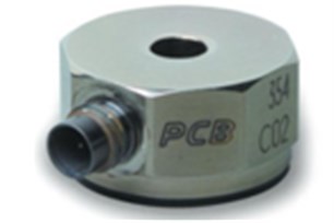
Fig. 2Detail of the axis directions considered

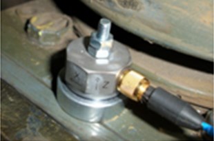
The accelerometer’s position is a major issue to consider. As it was studied by Weston et al. [12] three main movements can be observed: wheelset lateral motion, bogie motion and body motion. The first motion is the one that can give a closer behavior/performance to understand track irregularities because it is not affected by primary and secondary suspensions. Unlike in the vertical case, where the vertical displacements that the wheelset experiences are much closer to the vertical irregularity of the track than the vertical motion of any part of the bogie above; the lateral motion of the wheelset is not much closer to track alignment than the lateral motion of the bogie. This is the reason why, the study of lateral irregularities on the railway track can be made from the axle-boxes with the same precision as it would have if they were located in the wheelset itself. Therefore in this research accelerometers have been placed on the axle-boxes.

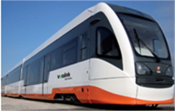
The vehicle used to do the measurements on the Line 1 was a VÖSSLOH-4100 that operates usually in this line. It can reach a maximum speed of 100 km/h. It has to be mentioned, that in the Alicante TRAM network tram-trains vehicles circulate thus combining tramway and train characteristics so the standards used to analyze the track quality should be approximated to this relatively novel combination.

Fig. 3Tram-train vehicle VÖSSLOH-4100

To complete the inertial monitoring system a Data Acquisition System (DAS) is necessary to collect and process all the information. “SARP MK2” was the DAS used for recording accelerations and was placed inside the train cockpit. A GPS (Garmin 18x-5 Hz) was employed to locate the train along the track and at the end to place all the results on the track route.

Fig. 4(a) Data Acquisition System “SARP MK2” and b) GPS Garmin 18x-5 Hz

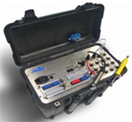
(a)

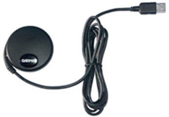
(b)

Accelerometers and GPS should provide data that must be compatible. Therefore both devices have to operate with the same sample frequency or at least data has to be treated to achieve it. Nyquist theorem [23] has to be satisfied. It states that in order to take a sample from a continuous signal, the frequency should be at least twice the maximum frequency observed. As maximum line speed is 100 km/h, accelerations are discretely recorder every 20 cm, so as to have data per meter which could be interesting for lateral alignment defects. The data obtained by the GPS show geographic coordinates (latitude, longitude, elevation) but as we are interested in comparison with the track monitoring trolley, the coordinates should be processed to the Universal Transverse Mercator (UTM) coordinate system. Once both data (accelerometer and GPS) are presented in homogeneous characteristics (spacing and frequency) data acquisition set-up has ended and data treatment is about to start.

4.2. Track monitoring trolley

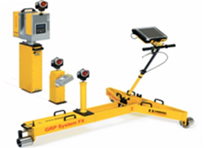
Data acquisition by track monitoring trolley is simpler than the inertial process. Lateral track profile has been obtained employing the GRP SYSTEM FX AMBERG track monitoring trolley. This trolley is a manually driven and measures different track parameters at the same time, providing an instant record of the track conditions and geometry. It is a high precision device although it requires service cuttings during monitoring tasks. Besides, as it is manually driven, the inspection takes much more time and the spatial range that can be measured is quite limited.

Fig. 5Monitoring trolley “GRP SYSTEM FX AMBERG”

The track monitoring trolley needs a robotic total station (Leica TRP in this case) to follow the trolley prism and therefore place all date registered in UTM coordinates. The robotic total station (RTS) locations require topographic information. This information was obtained from the topographic campaign made during the tramway line construction.

Once the different RTS placements are well known, the measurement process can be carried out. In the next table the whole process is described.

Table 1Track monitoring trolley measurement steps

Phase	Representation
PHASE 1 The trolley advances through the line. Its coordinates are taken from the RTS placed on the “Base 1”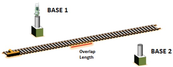
PHASE 2 The trolley reaches the end of the first track stretch measured by the RTS place on the “Base 1”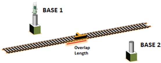
PHASE 3 The RTS is moved to the “Base 2”; meanwhile the trolley moves backwards approximately between 10-15 meters in order to create an overlap length and therefore avoid missing measurements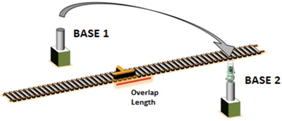
PHASE 4 The whole process is repeated again but each time from a different base location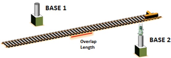

Once the measurement is done the recording data are already available. The only pretreatment that has to be made is the equally displacement representation of data, that means, obtain the data measured represented each 20 cm to be comparable with the inertial method. To obtain data equally displaced each 20 cm for both methods, an interpolation of the measurements has to be carried out. To do that spline interpolation has been selected as it gives the most approximated values.

5. Data treatment

In this point data treatment is completely described and the different steps taken are clearly differentiated. The main objective in this section is to, in a final stage, obtain with both data registrations (inertial and trolley) displacements that could be compared and this way be able to validate the proposed system.

The treatment sequence followed is explained in the next figure:

Fig. 6Data treatment steps

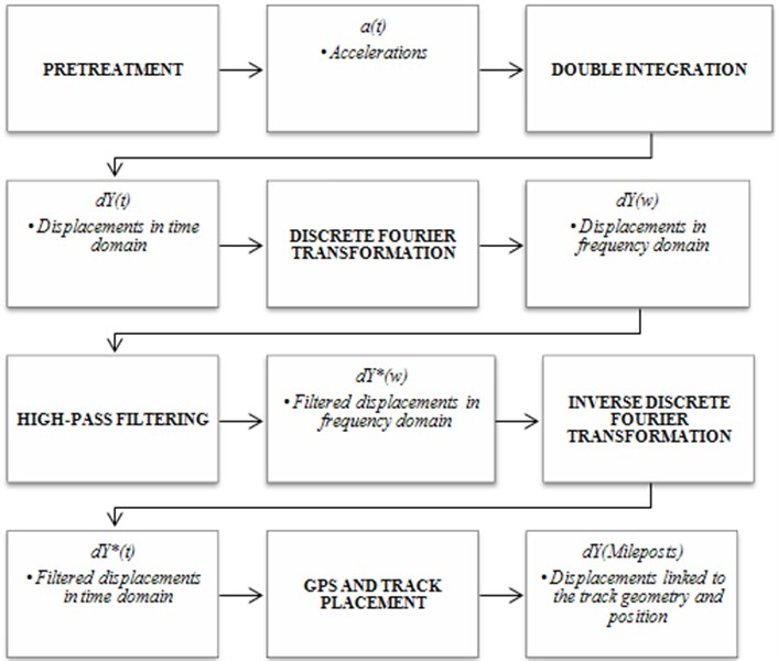
In the previous section, pretreatment was already explained so the next step to explain is double integration of the accelerations.

5.1. Accelerations double integration

As we need displacements to study track geometry quality, integration of accelerations has to be made. In this research lateral track irregularities are studied, so accelerations in the $Y$ – axis were analyzed.

Since acceleration data registrations were equally displaced each 20 cm they are a discrete recording. For this reason numerical integration must be applied. Trapezoidal rule of integration [24] has been implemented. It was checked that the integration error of this rule was under 0.1 % so the integration process is valid. However some difficulties appear during the integration process that must be corrected to avoid final results distortion. The effects of integration that have to be corrected are: reduction of high-frequency components, amplification of low frequencies and signal phase shifting.

The trapezoidal rule is expressed as:

1

I = \int_{a}^{b} f (x) d x \approx \int_{a}^{b} P_{1} (x) d x = \int_{a}^{b} (a_{0} + a_{1} x) d x = (b - a) \frac{f (a) + f (b)}{2} .

In order to prevent those inconveniences “baseline correction” technique was used. This technique lies in defining a function that has to fit data of the diagrams obtained (velocity and displacement) with certain accuracy. To ensure this precision level required least squares method is applied, then the resulting function approximates as better as it cans to the actual values. Moreover initial condition “zero velocity at initial instant” must be satisfied. It is a commonly used technique in seismic engineering [25] when accelerogram charts from an earthquake have to be analyzed.

Fig. 7Baseline correction of velocities

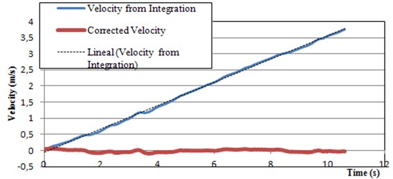
First velocity diagrams have to be adjusted by the baseline function and as difference with the original values “corrected velocity” is obtained. The baseline function can be: linear, polynomial, logarithmical, exponential among others. In order to know the goodness of the adjustment of each function $R^{2}$ parameter was observed. Polynomial 6th degree showed quite good results; providing values of $R^{2}$ always above the 95 %. It has also to be mentioned that a perfect adjustment will give the same values for the baseline function and therefore the “corrected” velocities or displacements will be all zeros.

The $R^{2}$ parameter is calculated as follows:

2

r = \frac{\sum (x - \bar{x}) (y - \bar{y})}{\sqrt{\sum {(x - \bar{x})}^{2} \sum {(y - \bar{y})}^{2}}},

where $x$ is the measured value, $\bar{x}$ is the measured mean value.

Regarding to the gauge analysis is important to understand that this geometric parameter measures the absolute distance between the rails independently of track geometry. That means that in the integration process previous acceleration values should not affect each registered data, so the implementation of the trapezoidal rule was a bit different:

3

v_{c} (i) = \frac{a (i - 1) + a (i)}{2} Δ t,

4

d_{c} (i) = \frac{v (i - 1) + v (i)}{2} Δ t .

In conclusion, double integration was done to obtain displacements from the acceleration registers. Once velocity is obtained at first integration, baseline correction function was implemented to obtain the “Corrected Velocity”. This adjustment was made with a 6th polynomial function. Then the “Corrected Velocity” data was again integrated and displacements were obtained. These displacements were also corrected with another 6th polynomial baseline function. At the end “Corrected Displacements” were obtained. For the gauge analysis, trapezoidal rule was modified considering its particular characteristics.

5.2. Filtering process

As it was mentioned before, frequency analysis allows a better study of the accelerations registered because with a filtering process different frequencies can be isolated and then the appropriated case study can be carried out in each situation.

As filtering is made in frequency domain, a previous step is to convert all data from time domain to frequency domain. The Discrete Fourier Transform (DFT) allows this conversion and its expression is as follows:

5

X (ω) = \sum_{r = 1}^{n} x (t) {exp}^{\frac{2 π i (r - 1) (s - 1)}{n}},

where $X (w)$ is the frequency domain signal, $x (t)$ is the original signal in the time domain, $I$ is the imaginary unit, $n$ is the data length and $r$ and $s$ are indexes varying from 1 to $n$ . The time domain is defined from $t_{0} =$ 1 to $t_{n} = T$ , being each value separated from $t$ obtained as $t_{r} = Δ (r - 1)$ , where $T$ represents the sample time length and $∆ t$ the time increment used when sampling; in this case equals to 0.01 s (corresponding to a 100 Hz frequency). In the frequency domain the interval goes from $w_{0}$ to $w_{n}$ taking the values:

6

ω_{s} = \frac{2 π}{T} (s - 1) .

The maximum wavelength belongs to the whole track stretch studied; and the minimum wavelength has to satisfy the Nyquist Sampling Theorem, so it belongs to the double of the sample frequency. Therefore the values of the wavelengths that limited the study are:

\begin{array}{l} λ_{m i n} = 0.40 m, \\ λ_{m a x} = 156.9 m . \end{array}

The length of 156.9 meters does not represent the length measured with the track monitoring trolley. Instead it represents the length of a smaller stretch of the track that is used to calibrate the model and then the results are extrapolated to the whole measured track.

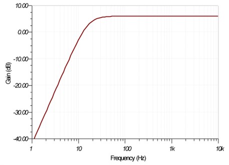
In this research as gauge and lateral alignment geometry parameters were analyzed, wavelengths between 3 and 25 meters were mainly studied. Therefore high frequencies must be addressed. In order to separate the frequency signal, so that high frequency components are visible and the others are neglected, a high-pass filter must be implemented. Then a high pass filter allows to pass all the high frequencies, from a defined “cutoff frequency”, and blocking all the frequencies below.

In the figure above a High-Pass filter response is represented. Ideal filters do not exist and then they are not reproducible and only a theoretical basis is given. It is physically impossible to obtain a zero bandpass transition between the passband and the stopband. Then a transition band between two frequencies is defined instead of one. This is why there is not only one Cutoff Frequency but two, and they are necessary to define the transition pass of the filter. Moreover what often occurs is that filtering operation is not uniform but it presents waves. They may appear in the bandpass and also in the transition band.

Fig. 8High pass filter response

As an ideal filter is impossible to obtain many approximations have been developed alongside filters evolution. Each approximation tries to be as closer as possible to the ideal filer by optimizing some of the parameters that define it. In this research Butterworth, Cauer and Chebyshev filters where employed and finally Butterworth results were the ones closer to the solution. Butterworth filter shows a quite flat response in the bandpass so the values which we are interested in will be nearly not affected. However the transition band is wider than other filters. The transference function is:

7

|H (j ω)| = \frac{K_{p b}}{\sqrt{1 + {(\frac{ω}{ω_{c}})}^{2 n}}},

where $K_{p b}$ is the gain of the filter, $ω$ is the frequency of each signal and $ω_{c}$ is the Cutoff frequency.

Fig. 9Butterworth performance. Differences between filter order values

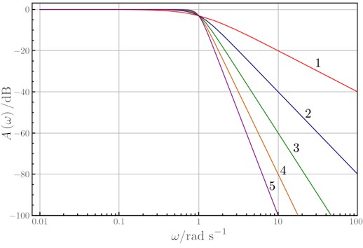
This figure shows the performance of a Butterworth filter for different values of “ $n$ ” (filter order). As the order of the filter increases the transition band decreases.

The type of filter that has been used, regarding to its way to operate, is an Infinite Impulse Response (IIR). This type of filters work with a recursive circuit, so feedback is provided. Their implementation is a bit more complex but uses less information and gives a better answer. The equation of an IIR filter is expressed as follows:

8

y [n] = a x [n] + a_{1} x [n - 1] + a_{2} x [n - 2] + \dots + a_{N} x [n - N] - b_{1} y [n - 1]

- b_{2} y [n - 2] - . . . - b_{M} y [n - M] .

This equation says that the output is function of the $N + 1$ sample inputs (the current one and the previous $N$ ), as well as the $M$ previous outputs obtained. The transfer function is the quotient between the $b_{i}$ and the $a_{i}$ .

As it was mentioned before, one of the integrations defects was phase distortion. To prevent that a phase correction function is defined as:

9

P (k) = \{\begin{array}{l} e^{i (a k - b - ϕ)}, & k < - k_{ϕ 0}, \\ 1, & - k_{ϕ 0} \leq k \leq k_{ϕ 0} \\ e^{i (a k + b - ϕ)}, & k > k_{ϕ 0}, \end{array},

where: $P (k)$ is the phase correction function, $k_{ϕ 0}$ is the cutoff wave number, $ϕ$ is the associated phase to each value obtained from the filtering process, $a$ and $b$ are parameters to calibrate the function.

This function leaves the phase unaltered for the wave number values between $- k_{ϕ 0}$ and $k_{ϕ 0}$ . For the values out of this interval the phase follows a straight line as the equation $ϕ^{*} (k) = a k \pm b$ explains. $ϕ^{*} (k)$ represents the new phase. The values of the parameters $a$ and $b$ must be obtained by an iteration process as well.

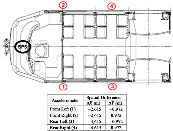
Fig. 10Accelerometers placement and spatial differences with the GPS location

Once the filter and the phase correction function are designed, the high frequency components of the original signal are obtained without any phase distortion. Then the conversion to the time domain is required, and to do so the inverse DFT is implemented:

10

y (t) = \frac{1}{n} \sum_{r = 1}^{n} Y (ω) {exp}^{- \frac{2 π i (r - 1) (s - 1)}{n}},

where $y (t)$ are the high frequency values with no phase distortion in time domain, $Y (ω)$ are the input values provided by the filtering process in frequency domain, $r$ and $s$ are values that go from 1 to $n$ , $n$ is the total number of values studied.

5.3. GPS and track placement

The last phase of data treatment consists of locating the displacement values obtained after the whole previous process in the track geometry. It is interesting that each displacement belongs with a Milepost value. This can be done by using the GPS records; besides the Milepost of a specific section of the track must be known. In this research, Milepost and UTM coordinates of Hiper Finestrat station were provided.

Hiper Finestrat Milepost and UTM coordinates:

MP. 40+038,230

$X$ : 746321 m

$Y$ : 4269795 m

Starting from this initial values, and considering that train speed is also known as well as the time increases between registers, each Milestone can be obtained as:

11

{M P}_{i} = {M P}_{i} - 1 + v_{i} (t_{i} - t_{i} - 1) .

The last step consists of a spatial transfer of data, since GPS is located on the cockpit front part. For each accelerometer the following spatial phase differences are shown in Fig. 5.

Fig. 11Gauge deviations. Comparison between the inertial system and the monitoring trolley

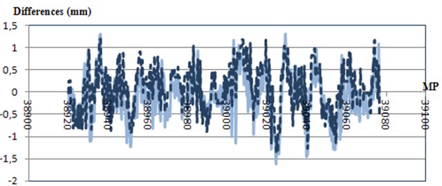
Fig. 12Lateral alignment deviations. Comparison between the inertial system and the trolley

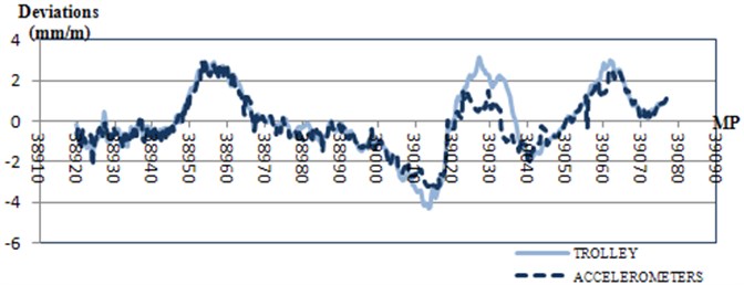
6. Comparison and validation

After data treatment it is possible to validate the proposed inertial monitoring system by comparison with the track monitoring trolley data. Two different comparison were made; at first an intuitive graphical comparison and secondly a more precise comparison based on statistic analysis.

6.1. Statistical comparison

However in order to ensure that the inertial system is enough efficient, a statistical analysis was carried out. Statistical comparison of both series was made regarding the Student’s T-test [26] and [27]. Null hypothesis is defined as the equality of both series Mean Value. A necessary condition to implement the T-test is that both series behave as a normal distribution. Normal distribution behavior and Student’s T-test were carried out by Statgraphics software.

Normal distribution behavior was confirmed for every distribution [gauge, lateral left alignment and lateral right alignment]. Therefore the Student’s T-test could be assessed.

Table 2Statistical analysis results

Statistic analysis	Gauge study ( $p$ -value)	Alignment study ( $p$ -value)
Mean comparison	0.4123	0.9999
Standard deviation comparison	0.0665	0.6544

All $p$ -values obtained are above 0.05, so the null hypothesis (equal mean values or equal standard deviation values) cannot be rejected. $p$ -values only express the rejection or not rejection of a hypothesis.

In conclusion, based on graphical and statistical results, the inertial monitoring system proposed is validated thus able to study track geometry quality.

7. Railway track quality study

Once the inertial monitoring system is validated, railway quality can be studied in the whole railway track measured. Spanish standards have been used to determine whether railway defects appear. Nevertheless, as it was mentioned before, urban and metropolitan railway vehicles have their own characteristics and speed ranges are quite different compared with conventional trains, so standards should be adjusted somehow.

Spanish standards employed were provided by UNE-EN 13848-1 [28]. Three range of wavelengths are defined to differentiate the various kind of defects on track.

$D 1$ : 3 m $< λ <$ 25 m

$D 2$ : 25 m $< λ <$ 70 m

$D 3$ : 70 m $< λ <$ 150 (200 for lateral alignment)

In addition three maintenance intervention levels are defined:

– Immediate Actuation Level (IAL): above these values measurements have to be carried out in order to avoid derailment risk.

– Intervention Level (IL): referred to the values that once exceeded, required corrective maintenance trying to foresee that IAL limits will not be reached on the next inspection.

– Alert level (AL): referred to the values that once exceeded, require that geometry track conditions were analyzed and regular maintenance tasks should be planned.

Then, considering the Spanish standards mentioned, it can be concluded that gauge defects were not present on this section of the line. Track monitoring trolley also conclude this so lack of accuracy is not the reason why there are not defects but only that the section studied is in good conditions (regarding to gauge parameter).

However, lateral track alignment analysis presents some points that exceed the threshold that has been used in this research: ±3 mm/m. Alignment defects are studied by meter because it gives a more realistic and accurate interpretation of the results.

Fig. 13Alignment deviations and standard threshold assumed

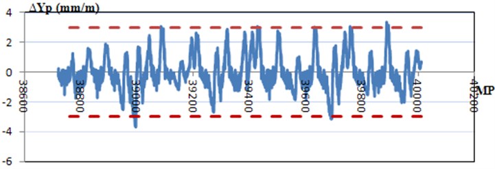
It is easy to obtain where the defects are because deviations are directly related with their Milepost value and therefore they can be located on the railway track.

8. Conclusions

In this research an inertial monitoring system has been proposed in order to detect and measure gauge and lateral alignment track defects. These systems record accelerations on the three main axes and after data treatment, reliable results have been obtained as it was explained and confirmed in the validation and comparison section. This inertial system was developed as a step forward in predictive maintenance.

Predictive maintenance provides many advantages; and the inertial method presented is able to do the continuous inspection that this maintenance requires. Services cuttings will be increased then transport offer quality will arise. Moreover safety conditions will be ensured since maintenance works will depend on track status, giving room for economic costs reduction.

Installation and data acquisition could be improved. Installation could be more sophisticated without the presence of hanging wires or duct tape. Data acquisition and treatment could be implemented automatically and direct results provided to a computer where track geometry status will be monitored continuously. Accelerometers are also an interesting tool to study passenger comfort, in this case they should be placed on the vehicle floor. Filtering process could be also optimized by reducing the iterative calibration of the parameters.

References

Zhang T., Andrews J., Wang R. Optimal Scheduling of Track Maintenance on a Railway Network.

Search CrossRef
Narayan V. Effective maintenance management – risk and reliability strategies for optimizing performances. New York, Industrial Press, 2004.

Search CrossRef
López Pita A. Railway Infrastructures. Barcelona, Ediciones UPC, 2006, (in Spanish).

Search CrossRef
Nagamuna Y., Kobayashi M., Nakagawa M., Okumura T. Condition monitoring of Shinkansen tracks using commercial trains. 4th IET International Conference Railway Condition Monitoring, Derby, UK, 2008.

Search CrossRef
Yazawa E., Takeshita K. Development of measure device of track irregularity using inertial mid-chord offset method. Quarterly Report of Railway Technical Research Institute, Vol. 43, Issue 3, 2002, p. 125-130.

Search CrossRef
Ahmadian M. Filtering effects of mid.chord offset measurements on track geometry data. Proceedings of ASME/IEEE Joint Railroad Conference, 1999, p. 157-161.

Search CrossRef
Toliyat H. A., Abbaszadeh K., Rahimian M. M., Olson L. E. Rail defect diagnsosis using wavelet packet decomposition. IEEE Transactions on Industry Applications, Vol. 39, Issue 5, 2003, p. 1454-1461.

Search CrossRef
Caprioli A., Cigada A., Raveglia D. Rail inspection in track maintenance: a benchmark between the wavelet approach and the more conventional Fourier analysis. J. Mech. Syst. Signal Process., Vol. 21, 2007, p. 631-652.

Search CrossRef
Kozek M. Track Quality Evaluation Using a Dynamic Black-Box Model of a Railway Vehicle: a Feasibility Study. Doctoral Thesis, Vienna University of Technology, 1998.

Search CrossRef
Coudert F., Sunaga Y., Takegami K. Use of Axle Box Accelerations to Detect Track and Rail Irregularities. WCRR, 1999.

Search CrossRef
Weston P. F., Ling C. S., Roberts C., Goodman C. J., Li P., Goodall R. M. Monitoring vertical track irregularity from in-service railway vehicles. J. Rail Rapid Transit, Vol. 221, 2007, p. 75-88.

Search CrossRef
Weston P. F., Ling C. S., Roberts C., Goodman C. J., Li P., Goodall R. M. Monitoring lateral track irregularity form in-service railway vehicles. J. Rapid Rail Transit, Vol. 221, 2007, p. 89-100.

Search CrossRef
Takeshita K. A method for track irregularity inspection by asymmetrical chord offset method. RTRI Report, Vol. 4, Issue 10, 1990, p 18-25.

Search CrossRef
Nagamuna Y. Track maintenance method considering dynamics of Shinkansen rolling stock. RTRI Report, Vol. 9, Issue 12, 1995, p. 37-42.

Search CrossRef
Carr G., Tajaddini A., Nejikovsky B. Autonomous Track Inspection Systems – Today and Tomorrow. AREMA, 2009.

Search CrossRef
Grassie S. L. Measurement of railhead longitudinal profiles: a comparison of different techniques. Wear, Vol. 191, 1996, p. 245-251.

Search CrossRef
Kawasaki J. Estimation of Rail Irregularities. Massachusetts Institute of Technology, 2001.

Search CrossRef
Bocciolone M., Caprioli A., Cigada A., Collina A. A Measurement System for Quick Rail Inspection and Effective Track Maintenance Strategy.

Search CrossRef
Mannara F., Barbati N. Acceleration measurement campaign on the bushings if a train ETR 220 from the Circumvesuviana railway track. Vol. 46. Issue 5, 2012, p. 449-467, (in Italian).

Search CrossRef
Tsunashima H., Nagamuna Y., Matsumoto A., Mizuma T., Mori H. Condition monitoring of railway track using in-service vehicle. Reliability and Safety in Railway, 2012.

Search CrossRef
Real J. I., Salvador P., Montalbán L., Bueno M. Determination of rail vertical profile through inertial methods. Journal of Rail and Rapid Transit, Vol. 225, Issue 1, 2010, p. 14-23.

Search CrossRef
Real J. I., Montalbán L., Real T., Puig V. Development of a System to Obtain Vertical Track Geometry Measuring Axle-Box Accelerations from In-Service Trains.

Search CrossRef
Smith S. W. The scientist and engineer’s guide to digital signal processing.California Technical Publishing, 1997.

Search CrossRef
Davis P. J., Rabinowitz P. Methods of Numerical Integration. San Diego: Academic Press, 1984.

Search CrossRef
Boore D. M, Stephens C. D., Joyner W. B. Comments on baseline correction of digital strong-motion data: examples from the 1999 Hector Mine, California, Earthquake. Bulletin of the Seismological Society of America, Vol. 92, Issue 4, 2002, p. 1543-1560.

Search CrossRef
Romero R. Engineering statistical methods. Valencia: Ediciones Universidad Politécnica de Valencia, 2005, (in Spanish).

Search CrossRef
Zimmerman Donald W. A note on interpretation of the paired-samples t-test. Journal of Educational and Behavioral Statistics, Vol. 22, Issue 3, 1997, p. 349-360.

Search CrossRef
European standardization committee. Railway applications. Track. Track Geometry Quality, Part 5: Geometrycal Quality Levels, UNE-EN 13848-5, 2009, (in Spanish).

Search CrossRef

About this article

Received

30 September 2013

Accepted

26 October 2013

Published

15 February 2014

Keywords

axle-box

accelerometer

alignment

maintenance

track monitoring

Acknowledgements

The authors of this paper would like to thank FGV Alicante personnel for their collaboration, interest and kindness during this research.

This is an open access article distributed under the Creative Commons Attribution License, which permits unrestricted use, distribution, and reproduction in any medium, provided the original work is properly cited.