Abstract
Free section friction on cantilever beam is the object in this paper. Practical experiment and virtual simulation are combined to gain understanding of the whole mechanical system. The classical Tustin model cannot provide perfect description of the actual friction process. Friction compensation model 1 is established through introducing time-varying compensation into the classical Tustin model based on the classical friction model and the theory of Fourier transform. A modified genetic algorithm is proposed by introducing self-adaptive strategy. The parameter identification based on the time-varying friction compensation model is performed by using the modified genetic algorithm. Friction compensation model 2 is established by introducing the improved time-varying compensation strategies which are more in line with the friction process. The numerical results demonstrate the high iterative search capability and computation efficiency of friction compensation model 2.
1. Introduction
Friction is generated by relative motion of non-ideal smooth contact [1]. It is a complex nonlinear physical process. Over the years, the study and analysis of the friction process has been a hot field in academe [2]. An accurate friction process model can play an important role in studies of mechanical system, structure optimization and friction compensation [3].
It is essential to choose appropriate models in processes of model parameter identification. Dynamic friction phenomenon cannot be described accurately by a classical friction model. Due to complex characteristics of a cantilever beam itself, traditional identification models of friction system cannot meet modeling requirements. The high-speed friction process studied in this paper makes it necessary to consider the impact of vibration on the cantilever beam in the titled direction. Therefore, an optimization identification model with time-varying characteristics compensation, which is named Augmented Tustin Model (ATM), is established based on the classical Tustin Model (TM) [4].
Many traditional optimization algorithms have been widely used in model parameter identification. These methods usually have their own limitations such as local convergence, inefficiency and easy to get into the local best. So, more attention should be taken to modern optimization methods for better solving capability. In the simulation section of this paper, an optimization algorithm with better convergence and global optimization functionality, which is named Modified Genetic Algorithm (MGA), is proposed by using self-adaptive strategy.
2. Friction identification model and intelligent algorithm
2.1. Experimental setup
The friction parameter identification is investigated for the sliding process of the moving mass. The experimental setup is shown in Fig. 1. The sketch of the motion is given by Fig. 2.
Fig. 1Picture of the experimental setup
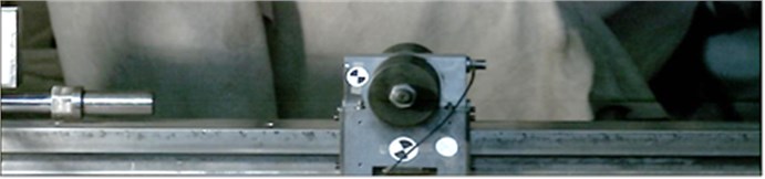
Fig. 2Sketch of the motion
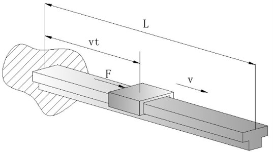
A pneumatic actuator is employed to drive the moving mass which can move along the cantilever beam at a certain speed (5-8 m/s). A high speed camera is used to record the motion with a sampling frequency of 4 kHz [5]. A low-pass filter is used to suppress the high frequency noise in the signal. By analyzing the motion images of the moving mass, the displacement, velocity and acceleration data is obtained. Since the mechanical stress analysis of the moving mass is the main issue, the acceleration data calculated from second order derivative of displacement is needed for further analysis. Based on friction identification model and intelligent optimization algorithm, the parameters of the friction model between the moving mass and cantilever beam will be obtained.
2.2. Tustin model
Based on Stribeck Friction Model, a static friction model can divide system friction into three parts [6]:
(1) Coulomb Friction (CF): The friction during the sliding process of a moving mass.
(2) Static Friction (SF): The friction which prevents a mass from static to dynamic.
(3) Viscous Friction (VF): The friction produced by viscous effect between interface materials.
The Stribeck Friction Model is expressed as:
where is total friction, is CF, is VF, is SF, is Velocity, is an experience parameter.
Generally, when 1, we get Tustin Model (TM), which is the most common Stribeck Friction Model. The TM is given by Eq. (2):
2.3. Augmented Tustin model
All the test accelerations in the experiments have sine characteristics, so it is essential to take sine components into account to improve TM, finally to get a more precise system friction model.
In this paper, the friction effect of the horizontal direction can be described by TM. But there are effects of other factors on moving mass, which can be compensated by using sine polynomials through the theory of Fourier transform. Owing to the limitation of numerical calculation efficiency, Augmented Tustin Model can meet the requirements when the exponent number of the sine polynomials reaches 3. There is a time signal t in the sine polynomial compensation which is also considered as a model parameter. To some extent, ATM can identify the time-varying characteristics of the free section friction on cantilever beam.
The time-varying friction compensation model ATM 1 is:
The three terms in Eq. 3 describe the effect of static friction, sliding friction and viscous friction respectively. In principle, static friction effect cannot be affected by external factors. However, sliding friction and viscous friction are the different cases. Though they are affected by the vibration and impact factors of the cantilever beam mechanism, the effects are not completely consistent. Therefore, sliding friction and viscous friction should be compensated respectively.
The time-varying friction compensation model ATM 2 is:
2.4. Genetic algorithm
Output signal of a time-varying system depends not only on input signal of the system but also on the moment of the input signal, which is different from output signal of a general constant system. The friction identification models in this paper are time-varying systems. Algorithm gain of conventional identification algorithms of a constant system, such as recursive least squares method, Newton iteration algorithm and Hessian gradient algorithm, will be close to 0 with the number of algorithm iterations increasing. Therefore, these algorithms do not have searching and iteration capability for time-varying parameters. Genetic algorithm (GA) is a kind of intelligent algorithm which has a strong iteration capability. GA will be used for the parameter identification in this paper.
Various advantages of GA are as follows:
(1) Self-adaption: the capability to adjust circumstance characteristics and disciplines when they change.
(2) Parallel calculation: decreases calculation expense to improve efficiency.
(3) Fitness function only: just needs a function to estimate individual fitness.
(4) Probabilistic conversion: conversion formula is flexible and probabilistic.
(5) Easily application: results from GA can be applied to solve problems directly.
(6) Several optimal solutions: GA gives a group of feasible solution.
2.5. Concepts about genetic algorithm
(1) Individual: entity with characteristics.
(2) Population: it is made up by several individuals, and individual number in this set is called population size.
(3) Encoding: for initial population of individuals, it must be encoded before computer calculation.
(4) Decoding: process converting coding space to solution space to find out optimal solution.
(5) Fitness: standards to estimate each individual’s fitness in current generation.
(6) Selection: choose better individuals to make up the next generation by certain probability.
(7) Crossing: two individuals are cut at the same position, then connecting crossly which make out two new individuals.
(8) Mutation: in each generation, individuals probably mutate to become a new one by certain regularity.
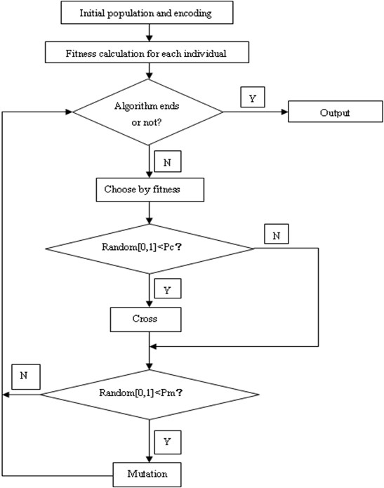
GA is a stochastic optimization technique inspired by genetic evolution mechanism [7, 8, 9]. It starts the search process from a set of randomly generated initial solutions which is called population. Each individual in the population is a solution to the problem, called chromosome. These chromosomes will evolve in subsequent iterations, and this process is heredity. GA is achieved by three aspects: crossover, mutation and selection. The operations of crossover or mutation will generate the next generation of chromosomes which are called offspring. The standard used to evaluate the quality of chromosome is called fitness, according to which a certain amount of individuals from current generation and offspring are chosen as the next generation of population to continue evolution. After several generations, the algorithm converges to the best chromosome, which is the optimal or suboptimal solution of a problem [10].
The iterative process of genetic algorithm is shown in Fig. 3.
Fig. 3Genetic algorithm flowchart
3. Case study
3.1. Analysis of TM
According to Eq. 2, there are four parameters to identify: , , and . In the experiment, pressure of 2 MPa and 3 MPa is applied respectively to produce the motion at two different speeds, which are low-speed group (4-5 m/s) and high-speed group (7-8 m/s). MGA is used for parameter identification. The identification results are as follows:
(1) Low-speed group (4-5 m/s):
(2) High-speed group (7-8 m/s):
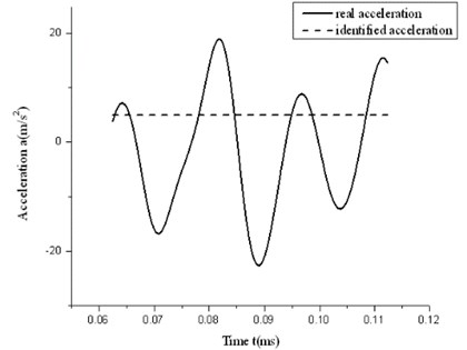
The test acceleration dithers obviously with certain degree of sine characteristics which is shown in Fig. 4 and Fig. 5. For high speed motion while friction is not significant, TM finds out easily that the friction or the acceleration is linear, as shown in Fig. 6 and Fig. 7. It is not ideal enough for current identification in real circumstance. Observing from the dithery test acceleration, we can learn that traditional TM is unsuitable for current system modeling. So existing classical models should be improved.
Fig. 4Low-speed acceleration trace
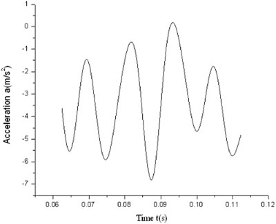
Fig. 5High-speed acceleration trace
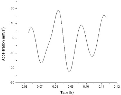
Fig. 6Result of low-speed group
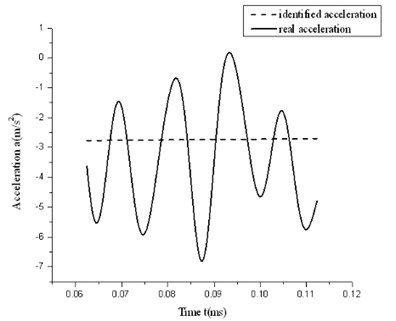
Fig. 7Result of high-speed group
Test acceleration curves of experiment are drawn in Fig. 8. It shows that all the test acceleration curves have sine characteristics, which means that the vertical vibration of the cantilever beam and the collision between the cantilever beam and the moving mass affect the motion of the moving mass in the horizontal direction. So it is reasonable to introduce sine polynomial compensation into TM.
3.2. Parameter identification of ATM
Pressure of 2 MPa and 3 MPa is applied respectively to produce the motion at two different speeds, which are low-speed group (5 m/s) and high-speed group (8 m/s). For the two friction compensation models ATM 1 and ATM 2, to distinguish the performance more accurately, the compensation orders of both methods are set to 2.
Fig. 8Test acceleration curves of experiment
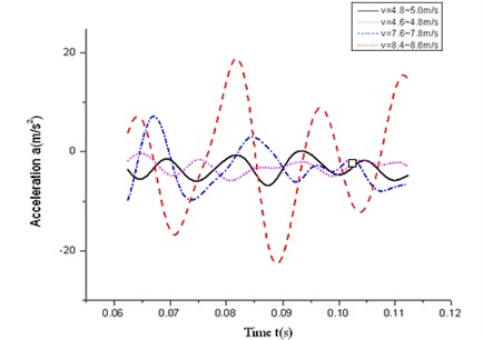
Table 1Results of low-speed identification
(N) | (N) | (N*s/m) | (m/s) | (N) |
29.9773 | 43.6321 | 4.7892 | 0.2881 | 38.2913 |
(N) | (rad/s) | (rad/s) | (rad) | (rad) |
151.2731 | 0.0198 | 0.0548 | -0.4921 | 1.0582 |
Table 2Results of high-speed identification
(N) | (N) | (N*s/m) | (m/s) | (N) |
32.3294 | 45.1892 | 6.8931 | 0.4219 | 42.3214 |
(N) | (rad/s) | (rad/s) | (rad) | (rad) |
182.3912 | 0.2031 | 0.0612 | -0.5391 | 2.0103 |
Fig. 9Low-speed acceleration curve
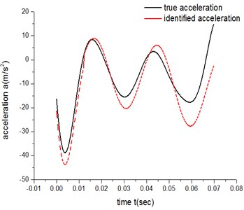
Fig. 10High-speed acceleration curve
For ATM 1, there are 10 parameters to be identified from Eq. 3 when 2. Table 1, Table 2, Fig. 9 and Fig. 10 show the results of identification for both the low-speed group and high-speed group.
The error of the low-speed group is 4.22×10³, while the result for the high-speed group is 8.06×10².
For ATM 2, there are 12 parameters to be identified from Eq. 4 when 2. Table 3, Table 4, Fig. 11 and Fig. 12 show the results of identification for both the low-speed group and high-speed group.
The error of the low-speed group is 1.37×10³, while the result for the high-speed group is 3.42×10². So ATM 2 for both the low-speed and high-speed group has a higher degree of accuracy than ATM 1.
Table 3Results of low-speed identification
(N) | (N) | (N×s/m) | (m/s) | (rad/s) | (rad/s) |
35.7298 | 42.7981 | 22.3214 | 0.6042 | 1.1021 | 1.9037 |
(rad) | (rad) | (rad/s) | (rad/s) | (rad) | (rad) |
1.4128 | 0.0653 | 2.1302 | 0.4902 | 0.7092 | 1.1932 |
Table 4Results of high-speed identification
(N) | (N) | (N×s/m) | (m/s) | (rad/s) | (rad/s) |
37.5031 | 47.3242 | 8.9972 | 0.5310 | 0.3402 | 0.9935 |
(rad) | (rad) | (rad/s) | (rad/s) | (rad) | (rad) |
0.0324 | 0.3801 | 1.5021 | 0.5921 | 0.2910 | 2.4532 |
Fig. 11Low-speed acceleration curve
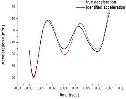
Fig. 12High-speed acceleration curve
It can be concluded from both the errors of low-speed groups and the errors of high-speed groups that, under the same experimental parameters and exponent number , ATM 2’s fitting degree of the actual friction process is higher than ATM 1’s.
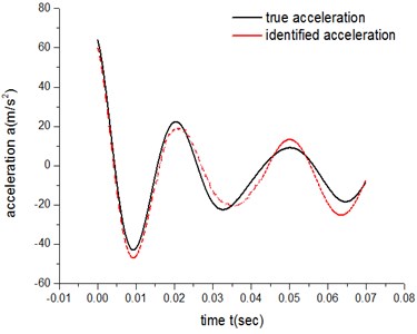
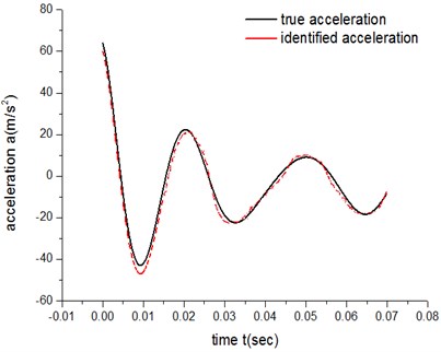
Based on the theory of Fourier series, when the exponent number of the sine polynomials increases high enough, the compensation term can help to process almost any signal precisely. That is, the errors of both ATM 1 and ATM 2 will be reduced with the exponent number increasing, and the results will be more accurate. In order to validate above analysis, two simulations under low speed condition were performed in which is 2 and 3 respectively.
Figs. 13-16 show that when the exponent number of the sine polynomials increases from 2 to 3, the identification accuracy of ATM 1 raise by about 9 %, which is much less than 300 %, the improved accuracy by ATM 2. It is because the compensation methods of ATM 1 is a merged compensation, where all other additional factors are merged together to form a compensation. The advantage of ATM 1 is that the exact physical meaning of compensation term does not need to be known a priori. But the flaw of merge compensation lies in adjustment and optimization flexibility of compensation terms, thus prevents further improvement of the identification accuracy.
Fig. 13Results of ATM 1 (N= 2)
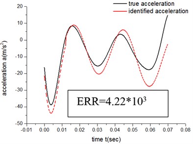
Fig. 14Results of ATM 1 (N= 3)
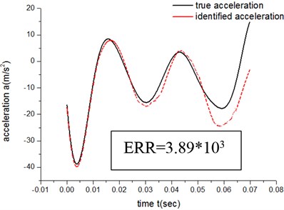
Fig. 15Results of ATM 2 (N= 2)
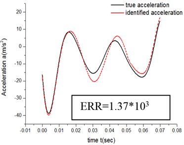
Fig. 16Results of ATM 2 (N= 3)
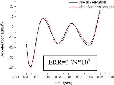
As mentioned before, the friction effect is divided into three parts: static friction, sliding friction and viscous friction. The effect of vibration and impact on these three parts is merged into a united expression in ATM 1. Static friction effect cannot be affected by external factors. However, sliding friction and viscous friction are the different cases. Though they are affected by the vibration and impact factors of the cantilever beam mechanism, the effects are not completely consistent. Accordingly the merged compensation model of ATM 1 will arise some identification error. Therefore, we proposed ATM 2, where sliding friction and viscous friction are compensated separately. Sliding friction and viscous friction are added by weight factors composed of sine terms. ATM 2 is more in line with the friction process description, which can make the accuracy better than that of ATM 1.
However, the exponent number of the sine polynomials increases by one, identification parameters will gain two at least. For ATM 2, if the exponent numbers of sliding friction and viscous friction both increase by one, four new parameters will arise. Too many identification parameters will significantly affect the performance of the algorithm. Accordingly, for the parameter identification of friction compensation model, it is important to select an appropriate compensation order number to ensure the balance of computation precision and efficiency.
4. Modified genetic algorithm (MGA)
Though the capability of GA is conspicuous, it holds inherent disadvantages. The shortcomings of GA include long identification time and low accuracy. How to avoid premature local optimum and increase convergence speed of the algorithm is the focal point of our study.
In order to enhance the efficiency of the algorithm and keep the diversity of each population, a self-adaptive strategy is introduced into the traditional GA. To improve the efficiency of the algorithm and ensure the population diversity and robustness, the probability of crossover operator () and mutation operator () are changed to self-adaptive parameters which are related with individual fitness and times of heredity.
A prior knowledge says that in GA, convergence rate and iterative efficiency are in very close contact with selections of crossover probability and mutation probability [11]. determines the amplitude of growth and searches new solutions of the population. A larger means stronger algorithm capability to open up new search range, which also means that better new individuals can be searched more easily and convergence rate of the algorithm can be accelerated. However, if is too large, searches will be random and function approximation and convergence capability will lost. Mutation probability is generally small, which maintains the diversity of the population and prevents the algorithm from running into local convergence too early. Searches will be completely random when is large enough. If is too small, the results may go into local optimum.
If the crossover probability is large in the early phases of iteration and small in the later stage, slow convergence or misconvergence can be inhibited effectively. The self-adaptive strategy of crossover probability is given by:
where is an curvature parameter, is convergence limit and is the number of iterations.
For different individuals in a population, mutation probability should be small for those having good target values and be large for those having bad ones in order to make the overall average fitness of the population good. The self-adaptive strategy of mutation probability is expressed as:
where is an curvature parameter, is the number of iterations, is optimal value, is average target value of the population, is individual target value and is adjustable constant of mutation probability.
The execution speed is crucial at the early stage of the algorithm but replaced by the precise optimal solution later. So the code length should be short at the early stage but long later. A changed critical point is set up at the position of 1/4 maximum number of iterations, where the code length remains unchanged. The self-adaptive strategy of code length takes the form of:
where is the coding constant, is the maximum number of iterations, is the number of iterations, is discrete curvature and is the code interval.
4.1. Analysis of MGA
In order to compare algorithm efficiency and capability to avoid local optima of GA and MGA, a trigonometric function of single target and multiple local extremum is adopted as a verification example, which is:
The size of the population is 40, while the code length is 20. The iteration is 200 generations and the fitness function is ordering distribution. A method of stochastic universal sampling is utilized for searching. The function diagram is given by Fig. 17.
Fig. 17Target value curve of the example function
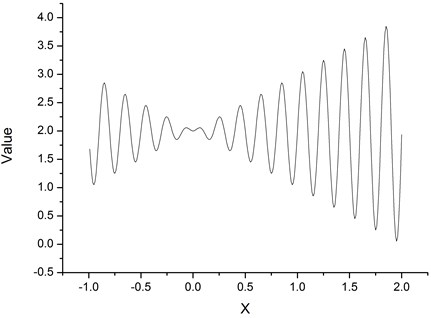
Simulation results (MATLAB) say that the maximum target value is 3.8503 and the corresponding is 1.8505. Because GA itself is an intelligent optimization algorithm with stochastic and probabilistic characteristics, 50 simulations were carried out for GA and MGA separately, among which the code length of MGA was a fixed number 20. The average value of the numbers, which represent the times of iteration to find the optimal solution, is chosen as a measure of the optimal iterative efficiency of the algorithm. Meanwhile, the execution time of each simulation is recorded to obtain the average time of these 50 simulations, which is also a measure of the calculation efficiency of the algorithm. The simulation results are shown in Fig. 18 and Fig. 19, in which the horizontal axis represents experiment amount and the vertical axis represents the time to obtain the optimal solution. Table 5 gives the efficiency of the algorithms.
Fig. 18Iteration times of GA
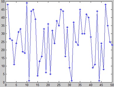
Fig. 19Iteration times of MGA
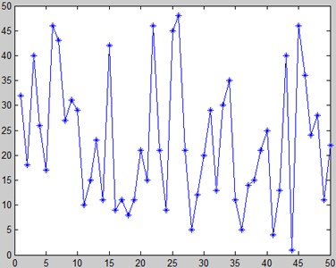
Table 5The efficiency of the algorithms
Algorithm name | Average times/generation | Average execution time/sec |
GA | 34.14 | 0.315051 |
MGA | 29.86 | 0.316321 |
The MGA introduces a self-adaptive method for crossover and mutation, which increases the algorithm complexity compared with GA. The average execution time is slightly longer (+0.4 %), while a stronger iterative capability can be obtained (the number of iterations decreases by 12.64 %).
Using the trigonometric function of Eq. 7, three coding ways, i.e. 10 bits binary code, 20 bits binary code and self-adaptive binary code, are adopted to test the algorithm performance in the iterative environment of 200 generations. The parameters of the self-adaptive binary code are: , , and . Execution performances of these three algorithms with different binary codes are given in Table 6.
Table 6Performance of three coding modes
Coding mode | Optimal value | Average execution time/sec |
10 bits binary code | 3.6792 | 0.184956 |
20 bits binary code | 3.8503 | 0.294762 |
Self-adaptive binary code | 3.8503 | 0.210445 |
Table 6 reflects that the self-adaptive binary code maintains the global optimal. It not only has the same accuracy with the fixed number binary codes, but also has higher execution efficiency than the fixed number binary codes. Therefore, the self-adaptive coding strategy contributes to effective balance of the execution efficiency and accurate search capability.
The proposed MGA is an optimized algorithm. In order to test whether it has optimized performance, 50 contrast experiments in which the traditional GA and the MGA with the self-adaptive binary code were utilized were conducted. The main algorithm performance comparisons are listed in Table 7.
Table 7Performance comparisons
Name | Average iterations | Average time/sec | Local optimal probability |
GA | 689.22 | 15.2982 | 30 % |
MGA | 479.86 | 9.3094 | 6 % |
It declares that for the friction process of the free motion on cantilever beam, introducing multiple self-adaptive strategies into optimize GA guarantees higher algorithm efficiency based on high identification precision.
5. Conclusion
All the acceleration curves at different speeds in this paper have significant sine characteristics. The vertical vibration of the cantilever beam and collision between the moving mass and the cantilever beam affect the motion in the horizontal direction to a certain extent. Traditional Tustin model cannot provide good actual description for the friction process. Through extension and compensation by adding sine polynomials in the traditional Tustin model, an augmented Tustin model is established which can improve the identification accuracy effectively.
ATM 2 has better identification accuracy than ATM 1. When the exponent number of the sine polynomials increases, the identification accuracy improved by ATM 2 is higher than that of ATM 1. With the exponent number increasing, the identification precision will be improved. However, a larger leads to a slower calculation speed. When is 2, the parameter identification accuracy can be guaranteed well.
The genetic algorithm is improved by determining the dynamic crossover probability , mutation probability and coding bits with self-adaptive strategy. The MGA can improve the iterative search capability and computation efficiency significantly.
References
-
Shousong Hu Automatic control theory. Science Press, Beijing, 2007.
-
Yuankai Yang, Xuying Lang Dynamic compensation of friction torque in precision turntable. Acta Automatica Sinica, Vol. 9, 1983, p. 248-252.
-
Jiajun Zou, Yanling Xing, Lanbing Mao Nonlinear system parameter identification of wavelet method. Suzhou University Journal, Vol. 29, Issue 1, 2009, p. 68-733.
-
Cadunas C., Astrom K. J., BraunK. Adaptive friction compensation in DC-motordrives. IEEE J. Robot. Automat RA, Vol. 3, Issue 6, 1987, p. 681-685.
-
Sanxi Zhang, Min Yao, Weiping Sun High speed camera and its application technology. National Defence Industrial Press, 2006, p. 27-34.
-
Saleem A., Wong C. B., Pu J., Moore P. R. Mixed-reality environment for frictional parameters identification in servo-pneumatic system Simulation. Modeling Practice and Theory, Vol. 17, 2009, p. 1575-1586.
-
Zhenchao Wang, Haibin Duan, Xiangyin Zhang An improved greedy genetic algorithm for solving travelling salesman problem. International Conference on Natural Computation, 2009.
-
Taboada A., Espiritu Jose F., Coit David W. MOMS-GA: A multi-objective multi-state genetic algorithm for system reliability optimization design problems. IEEE Transactions on Reliability, Vol. 57, Issue 1, 2008.
-
Youngjun Ahn, Jiseong Park, Cheol-Gyun Lee, Jong-Wook Kim, Sang-Yong Jung Novel memetic algorithm implemented with GA and MADS for optimal design of electromagnetic system. IEEE Transactions on Magnetics, Vol. 46, Issue 6, 2010.
-
Huijun Guo, Junhua Liu Identification of chaotic systems based on GA-Fuzzy. Journal of System Simulation, Vol. 16, 2004, p. 1323-1326.
-
Hua Chun, Haizhen Wang Analysis of the principle and constitute of the genetic algorithm. Journal of Inner Mongolia University for the Nationalities, Vol. 6, 2009, p. 632-634.
About this article

The authors would like to acknowledge the financial support from project Major State Basic Research Development Program of Republic of China.
