3-D calibration method and algorithm for freehand image of phased array ultrasonic testing

2.1. Theory of calibration algorithm

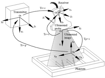
Figure 1 is the spatial relationships of the devices of the 3D phased array ultrasonic calibration system. The calibration is a procedure to calculate the spatial transformation relationships between the US probe coordinate system and the tracker coordinate system $T_{r\leftarrow i}$. Current tracking sensors mainly include the magnetic tracker and the optical tracker. We selected the magnetic tracker which was also called magnetic receiver. When select the magnetic tracker, the metal influence of the magnetic field must be considered, because the ultrasonic testing is different from the medical ultrasound, its probe usually is manufactured with metal and it is probably used to test the metal materials.

Finally the image calibration $T_{r\leftarrow i}$ is the matrix:

Fig. 1Coordinate systems definition and transformation relationships include receiver transmitter, receiver, phantom and image coordinate systems

2.2. Phantom and ${\mathit{T}}_{\mathit{p}\leftarrow \mathit{t}}$ calibration

In order to obtain $T_{r\leftarrow i}$, $T_{p\leftarrow t}$ must be required. $T_{p\leftarrow t}$ can be obtained by using the probe to scan a phantom with special geometric characteristic points. As is presented in Figure 2, we design a cross-string phantom which is consisted of cross-string, their planar arrays and phantom frame. The cotton strings of the cross-string are 0.3 mm in diameter. Because of their elasticity, they can keep tightened to maintain the string’s position precision both in dry and wet conditions in water. The cotton stings pass through the holes, 1 mm in diameter, on both front and back walls of the phantom frame. There are two layers of cotton strings arrays in the middle of the phantom frame.

Fig. 2Phantom construction and coordinate systems definition

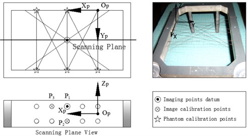
The 10 holes in the two opposite sides of the phantom frame which are the endpoints (holes) of the ten vertical strings passing through the phantom are characteristic points for the phantom calibration (Figure 2). They are marked as the stars, double 2 endpoints in the up side and double 3 endpoints in the down side. The phantom calibration is as followings. All coordinates of the marked points in the phantom coordinate system $P_p$ are given when the phantom is designed. Place the needle attached with the tracker (magnetic receiver) at the characteristic holes on the phantom, through magnetic tracking algorithm $T_{t\leftarrow r}$, the coordinates of these holes in $Ot$ (the magnetic transmitter coordinate system) are be calculated, marked as $P_t$.

2.3. Imaging

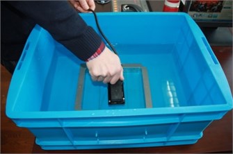
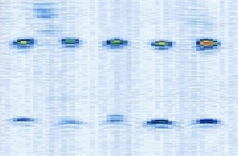
Place the US probe upon the cross-strings align with the middle string cross planar arrays (Figure 3), adjust the probe’s orientation and position, to ensure the ultrasound plane aligning with the cross-string layers. Until the 10 middle points are all in the US image, two layers, 5 imaging points in each layer, total 10 imaging points are shown. In this procedure, the strings trend nearby the middle cross arrays are help the probe find the middle cross arrays rapidly. The image origin is defined at the top centre of the sector surface of the US image (Figure 3).

Fig. 3Probe scanning and ultrasound imaging Place the probe upon the middle crosses planar of the strings and ten lightened points in the US image

a)

b)

2.4. Image calibration algorithm

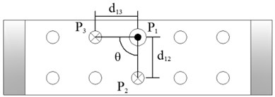
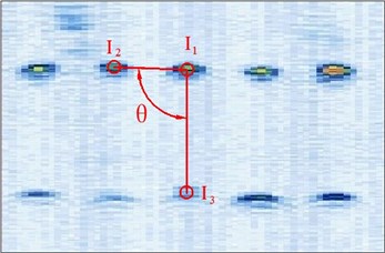
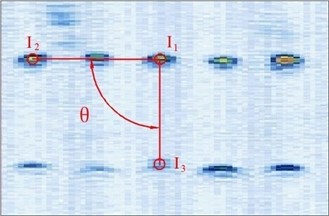
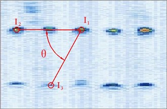
Figure 4 shows the image calibration algorithm. There are ten imaging points in the ultrasound probe scanning image. They are the corresponding images of the cotton strings crosses in the phantom. The algorithm concerns about two points’ coordinates, and they are $I_1$ and $I_3$ (Fig. 4(b)). The coordinates of $P_1$, $P_2$, $P_3$, $d_{12}$ and $d_{23}$ in the phantom are known by design, so the angle $\theta$ between $\stackrel{-}{P_1{P}_3}$ and $\stackrel{-}{P_1{P}_2}$ can be calculated by $P_1$, $P_2$ and $P_3$ (Fig. 4(a)). Then $\theta$ with the distances $\mathrm{}{d}_{12}$ and $d_{23}$ provide three parameters for calculating the image point $I_2$ and $I_3$.

Fig. 4Image calibration algorithm: a) Homologous points and matching parameters in phantom; b) Homologous points in image and algorithm

a)

b)

The calibration procedure is as followings:

(1) Manual mark $I_1$. $I_1$ is the middle imaging point of the middle cross $P_1$ of the up layer of the ten crosses in the phantom. In this algorithm $I_1$ is elected as the reference point, because it is nearby the centre line of the sector region in the US image. As the reference of the other points, the distances between other points and it should be calculated. $I_1$ in the image and $R_1$ in the receiver are the two homologous points. Where $R_1$ in the receiver in the receiver is calculated by $R_1=T_{r\leftarrow t}\cdot T_{t\leftarrow p}\cdot P_1$. Mark ten times repeatedly and average them as the result of the reference coordinate.

(2) Manual mark and calculate $I_2$. $I_2$ is a point near the reference point $P_2$ of the layer below of the ten points sequence in the scanning image. The algorithm requires to mark the highlight point below the reference point $I_1$, thus the direction of the vector $\stackrel{-}{I_1{I}_2}$ is obtained. Then calculating the distance from $I_1$ to $I_2$ according to $d_{12}$ (be converted to pixel). Which is determined by the crosses distance in the phantom. $I_2$ in the image and $R_2$ in receiver are the two homologous points. Where $R_2$ in the receiver is calculated by $R_2=T_{r\leftarrow t}\cdot T_{t\leftarrow p}\cdot P_2$.

(3) Calculate $I_3$. $I_3$ is a point near the left side of the reference point $P_3$ along the vector $\stackrel{-}{I_1{I}_3}$. The direction of $\stackrel{-}{I_1{I}_3}$ is calculated by $\stackrel{-}{I_1{I}_2}$. And the distance from $I_1$ to $I_3$ can be calculated according to $d_{13}$ (be converted to pixel). Which is determined by the crosses distance in the phantom. $I_3$ in the image and $R_3$ in the receiver are the homologous points. Where $R_3$ in the receiver is $R_3=T_{r\leftarrow t}\cdot T_{t\leftarrow p}\cdot P_3$.

(4) Apply the least-square fitting to $P_r\left(R\right)$ and $P_i\left(I\right)$:

where $s$ is the coefficients of the image (scales, mm/pixel). Calculate the transformation matrix $T_{r\leftarrow i}=(R,p)$ ($R$: rotation matrix, $p$: translation vector) by the theory of finding the minimized distance between the homologous points $P_r$ and $P_i$ [7]. $T_{r\leftarrow i}$ is a 4×4 matrix (rotation, translation and scale) shown as Eq. (3). Its first three columns form $R$ and the fourth column forms $p$.

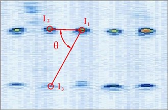
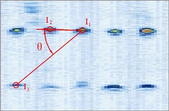
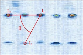
(5) Select different distances points from the reference $I_1$ as the algorithm $I_2$ and $I_3$ like Figure 6, repeat (2)-(4). Then average the calibration matrixes as the ultimate result $T_{r\leftarrow i}$.

The calibration matrix can be calculated from a single US image. However, due to the variations when the probe is placed upon the phantom to find the scanning plane with freehand scanning mode, the final calibration matrix is calculated based on 4 images repeated the manual marking and coordinates calculation. Then use each mass center of the homologous points to calculate the transformation matrix. In each US image, the two imaging points are manual marked by our self-developed software.

3.1. Calibration precision

The first calibration evaluation method was formulated by Detmer et al. (1994) and used by various other research groups (Leotta et al. 1997; Prager et al. 1998; Blackall et al. 2000; Meairs et al. 2000; Muratore and Galloway Jr. 2001; Brendel et al. 2004; Dandekar et al. 2005). Reconstruction precision is measured by the spread of the cloud of points. But the reconstruction precision measures the point reconstruction precision of the entire system, rather than calibration itself. This is dependent on a lot of factors, such as position sensor error, alignment error and segmentation error [7].

So we apply the measure, based on the same idea as above reconstruction precision, is called calibration reproducibility (CR) [7]. Calibration reproducibility measures the variability in the reconstructed position of points in the receiver’s coordinate system. This method is not necessary to reconstruct the point in world space, since the transformation $T_{t\leftarrow r}$ is independent of calibration, so it avoids variations of position-sensing. If we assume that a point has been imaged without scanning such a point physically, and that its location $P_i$ have been perfectly aligned and segmented in the images. Calibration reproducibility is calculated as follows:

where, the measure for calibration reproducibility depends on the calibrations $T_{r\leftarrow i}$ and the point $P_i$. From 1998 Prager chose $P_i$ to be the center of the image, and was quoted by Leotta in 2004 and the Cambridge group (Treece et al. 2003; Gee et al. 2005; Hsu et al. 2006). Some researchers also gave the variation at the same method as Prager, such as Meairs in 2000 and Lindseth in 2003. Pagoulatos proposed variations based on multiple points middle-down of the image in 2001. However subsequent research of Hsu in 2009 found that the errors measured by points towards the edges are more visible than that near the center of the image. Therefore many papers quote calibration reproducibility for a point at a corner of the image recently, such as Blackall in 2000 and Rousseau in 2005. Leotta in 2004 measured errors by points along the left and right edges of the image. The four corners of the image is another method implemented by Treece in 2003, Gee in 2005, Hsu in 2006 and Hsu et al. 2009. Brendel in 2004 gave the maximum variation of every point in the B-scan. Calibration reproducibility is only relative to calibration results, and does not incorporate errors like the sensor performance or human factors such as alignment and segmentation. Therefore calibration reproducibility has been considered as the evaluation standard when precision is measured.

Fig. 5Different manual points for image calibration

a)

b)

c)

d)

e)

So in this article, the calibration reproducibility is the method to evaluate the calibration precision. The points $P_i$ were marked at the four corners of the image. The calibration reproducibility is in a matrix [7]. The major factors causes the variations of the elements of calibration are: 1) Positioning errors when the stylus being placed into the hole on the phantom during phantom calibration (stylus measurements); 2) Placement incorrect when the phantom scanned by the probe freehand (phantom imaging or probe alignment); 3) Manual errors of the pixel coordinates of the crosses in the US image (manual image marking or segmentation). In the past researches, the third aspect is the most difficult to decease the errors. In our experiment, except for the method of homologous points in Figure 5, we select the points with different distances and angles to the reference point to calculate the matrix and average them as the final calibration matrix.

Repeat each of above three operations 10 times and computing variations of the calibration matrix. The probe was moved away from the strings and repositioned for each of the 4 images. This method ensures the independency of each image collection and presents the actual precision of the repeated calibration. The results are shown in Table 1. The first six rows are the rotation matrix elements and the last three rows are the translation vector in millimeters. The third column of calibration matrix is not shown, because it is the cross-product of the first two columns. The maximum discrete degrees are from 1.8696 mm to 2.6299 mm, it is show that the alignment of the probe procedure is the largest influence for the calibration precision. This is mainly caused by the ultrasound width. The calibration precision shows the same as other published methods reviewed by Hsu in 2009.

Points every 30 pixels were selected along the center and edge of the US images. Then translate these points in each image into the 3-D coordinate system, and then calculate the $\mathrm{\Delta }{P}_{CR}$, evaluating the point reconstruction accuracy. Repeat 10 times in phantom imaging, manual image marking and stylus measurements. The root mean square (rms) variation, the vector sum of the standard deviations SDs in the $x$, $y$ and $z$ direction, in the reconstructed pixel locations is a measure of the repeatability of the calibration method. The results are shown in Table 2. The calibration variability caused by image marking and stylus measurement was less than that caused by probe alignment. The calibration variability was higher when the depth is larger.

3.2. Reconstruction accuracy

One popular method for reconstruction accuracy is point reconstruction accuracy, which develops with the increased use of the stylus. Scan a point firstly, then calculate its 3D reconstructed location based on the calculation results. The 3D location of the point can be tested through the stylus, and the operation like in the Figure 3. This method was used transforming the points into the world coordinate system by Blackall in 2000, Muratore and Galloway Jr. in 2001, Pagoulatos in 2001 and into the sensor coordinate system by Lindseth in 2003. The discrepancy between the reconstructed coordinate and the stylus reading of the point reflects the reconstruction accuracy, i.e.:

This measurement includes errors from every component of the whole system. The thick beam width is the main causes for the error of the scan plane manual misalignment when using the point phantom. And segmentation error and position-sensor error are also the sources of error. So the point should be scanned from different positions and at different locations in the B-scan. A large number of images should be captured and the results averaged [7]. The other, the same phantom and the same algorithm are not very appropriate to used assessing the point reconstruction accuracy, because the phantom errors or the algorithm errors will cause an offset in the calibration. These offset errors are easy to be neglected.

The other popular method for reconstruction accuracy is distance reconstruction accuracy, which is used before the stylus was developed. Many groups through measuring the distances between two points in 3D space and compare them with the distances in the phantom to obtain the reconstruction accuracy, such as Leotta in 1997, Prager in 1998; Blackall in 2000, Boctor in 2003, Lindseth in 2003, Leotta in 2004, Dandekar in 2005, Hsu in 2006, Krupa 2006. When using this method, we should note that the line image will be a distorted curve for line image calibrations, and the distance between the two end-points will be incorrect. So in this research we rotated the probe in different directions when scanned the phantom. The discrepancy between the reconstructed distance and the phantom distance of the two points reflects the distance accuracy:

Therefore, the repeated precision reflects the stability degree of the calibration matrix, but does not provide an estimate of the validity of the calibration matrix, the effect of its 3-D transformation, so the point reconstruction accuracy and the distance reconstruction accuracy evaluation are necessary. The method is: rotate the probe in different directions when scanned the phantom. Apply the calibration matrix to translate the three point, $I_1$, $I_2$ and $I_3$, calculate the distance between $I_1$ and $I_2$, $I_1$ and $I_3$, then compare the distances with the real distances in the phantom. These data reflect the relative reconstruction accuracy. The experiment was divided into two groups, C: repeat the above to two procedures using the center 2 points to calculate the reconstruction accuracy, A: repeat the above to two procedures using the middle 4 points to calculate the reconstruction accuracy and B: repeat the above to two procedures using the edge 4 points to calculate the reconstruction accuracy. The results as seen in Table 3 show that the reconstruction accuracy of the center points is similar to that of the edge points. The point reconstruction accuracy is under ±0.15 mm.