Abstract
Reliable use of -value in is critical in seismicity comparisons, seismic hazard analysis, prediction and comparative mechanism studies. Since earthquakes and the -value are considered as stochastic processes and random variable, respectively, applying the probability distribution of -value is necessary in its temporal and spatial variations assessment. In this paper, we propose a novel method that employs the -value uncertainty in probabilistic seismic hazard analysis using normal-exponential joint distribution function. To this end, we calculate -value statistics based on bootstrap sampling of the seismic catalog. Our analytical and experimental evaluations show that the proposed joint distribution results in a more precise closed-form relation for the probabilistic seismic hazard analysis accurately reducing the hazard in comparison to conventional methods. The benefit of the proposed approach here is improving the ability of assessing the effectiveness of various seismic risk mitigation strategies and so, allocates the available resources more efficiently.
1. Introduction
Probabilistic seismic hazard analysis (PSHA) estimates the probability that the ground motion exceeds a specified level in a certain location and time period. PSHA methods compute the likelihood of an aggregated hazard based on source model, recurrence model and attenuation relationships. The hazard is generated from the occurrence of earthquakes with various magnitudes in different distances. Therefore, the variability of the earthquake magnitude, location (source-to-site distance), and ground motion level (denoted as the number of logarithmic standard deviations from the logarithmic mean) are considered in the hazard calculation [1]. The inherent variability considered directly in the PSHA calculation is called the aleatory variability.
Recurrence models provide cues to future earthquakes based on past earthquakes information and statistical assumptions. These models are divided into two categories; inter-arrival time and magnitude distribution models. Gutenberg-Richter law (G-R law), characteristic size model, and slip predictable model are examples of the first category, and Poisson model, characteristic time model and time predictable model lie in the second one that all suffer from uncertainty in their model and parameter calculation, called the epistemic uncertainty. Usually, the model uncertainty is regarded using the logic tree [2].
The G-R law, that represents the earthquake frequency, is one of the most significant and universal features of global seismicity [3]. The usual form of this law is written as:
where is the number of events with magnitude not less than , and and are constant coefficients. This equation gives the distribution of earthquakes in terms of magnitude, i.e., the distribution function in the magnitude domain. The G-R law is considered versus independent rates in every magnitude interval.
The value of the slope in the Eq. (1), i.e., the -value, gives a measure of the relative frequency of lower and higher magnitude earthquakes. It is also a well-known influential variable in seismic hazard analysis and structural design [4, 5]. High -values show that a small fraction of the total earthquake events in a region has high magnitudes, whilst low b-values indicate a large fraction of high magnitude events. The -value is inversely proportional to the mean magnitude of earthquakes:
where and are the minimum and mean magnitude in the dataset, respectively. Hence, the diagram of -value is equivalent to that of the mean magnitude [6]. In the seismic-prone region evaluation, comparison of -values is more understandable than other parameters [7].
-value is not a single unvarying amount. Different investigators give different -values in the same region [8]. Gutenberg and Richter propose to use -value equal to 1 for the whole world or large volumes. The -value estimation at different regions has been the subject of many scientific researches. In many cases, the results of these researches give other values for -value [9]. Shi and Bolt studied the uncertainties in the -value estimation [10]. They considered -value as a random variable. Some seismologists have firmly emphasized that -values are empirically constant, within the limits of statistical variation for the earthquake. Therefore, it is believed that the statistical fluctuations or observational uncertainties have the main responsibility in the variation of the -value.
Accurate estimation of the magnitude cumulative distribution function is necessary for the PSHA [11]. Thus, the rational method can be considered as the approach that can apply calculation errors to parameters beside their estimation. In order to apply the uncertainty in PSHA, the analytical methods are more appropriate than the numerical ones. Cornel believed that the main advantage of an analytical approach (i.e., the closed-form equation) over numerical solutions is that the sensitivity of the hazard curve to the parameters can be evaluated directly [12].
In this paper we propose a closed-form method to incorporate the estimation uncertainty in PSHA formulation using Bayes' theorem. We identify -value uncertainties and determine their distribution to incorporate quantitatively in the hazard evaluations. Then, we rewrite the PSHA formulation and derive a statistical model containing the parameters uncertainty (i.e., the uncertainty of -value and magnitude) based on a normal-exponential distribution. Finally, the effect of the proposed method on the hazard curve is studied using practical examples of some fault with different maximum magnitudes, lengths and source-to-site distances.
2. -value uncertainty resources
In the classic PSHA, under the assumption of Poisson distribution, seismic hazard is expressed as the probability of an earthquake intensity measure (such as peak ground acceleration ()) exceeding a threshold value [13]:
where is the threshold value, is the joint probability density function (PDF) of earthquake magnitude (), source-to-site distance (), and uncertainty () [14], and is expressed as:
In this relation, , , and are random variables, is the PDF of , and and are conditional PDF of and , respectively. Seismic sources are usually assumed with a capacity to produce some maximum magnitude . On the other hand, for engineering purposes, very small magnitude earthquakes () that cannot damage the structures are not of interest. So, in practice, experts usually use the truncated exponential model as . This model represents the truncation of the G-R law as:
where .
Although PSHA promises to provide a framework in which decision makers can be presented with a quantified range of possibilities, the above equations do not consider recurrence relationship uncertainty in the computation. G-R law parameters are obtained using regression analysis. Krinitzsky states several reasons for -value fluctuations, such as differences in the boundaries selected for the source, whether the earthquake tabulation are cumulative or non-cumulative, different normalizations of the information, additions of data to the earthquake catalog, processing of the catalog to eliminate duplicate listings, aftershocks and noises [15]. The causes of output uncertainty can be categorized as input uncertainty, model uncertainty and regression uncertainty. The first category (i.e., earthquake catalog uncertainties) includes uncertainties related to earthquake location, time and magnitude. The second category contains uncertainties resulted from model assumptions which can make the process easier. Some of these assumptions, which are later proved to be mistakes, are the major factors in model uncertainty. Thus, more accurate model assumptions will increase the model reliability. For example, G-R law is based on the assumption of an exponential relationship between the frequency and magnitude. Thus, if the region seismicity is not consistent with this presumption, the G-R law excludes the part of data which doesn’t fit to assumption. This may cause real earthquake scaling information to be lost and the uncertainty to be increased. Lombardi shows that if the data doesn’t follow the assumed exponential distribution, the simple maximum-likelihood (ML) estimator will give a totally different -value [16]. Also, the use of continuous models for rounded observation values lead to biased estimates [17]. The third category includes regression and parameter estimation uncertainties. Regression models (e.g. linear ones) are used for seismicity parameter assessment based on available seismic data. Linear regression methods find the best-fitting straight line through the existing points. The random scatters around the line (a.k.a., residuals) are identified as the distance of each point from the fitted line. In the next section we elaborate the role of residuals in PSHA.
Shortly, three strategies have been followed for uncertainty reduction in PSHA, namely, re-evaluation of inputs, using best models, and considering calculation errors. In the present paper, we propose a method to modify PSHA model regarding the statistical uncertainties in the G-R recurrence model parameter (-value).
3. Methodology
As discussed previously, despite the importance of parameter uncertainty the classic PSHA method does not treat it correctly. Here we propose an approach to consider -value statistical variation based on its distribution function. This approach assumes seismic events as independent, identically distributed random variables.
The observed -value is distorted by an observational stochastically independent error . The error is supposed to be normally distributed with the standard deviation [18, 19], i.e., , where is the normalized residual which is a normal distribution parameter with a constant standard deviation of 1. Therefore, is the number of standard deviations by which the -value deviates from the predicted one.
The -value (or ) is calculated using regression analysis. Based on the assumption of normal residuals, and taking it as random variable [20], its normalized residuals () have a probability distribution as follows:
where states the distribution of and denotes the normal distribution with average and standard deviation of and , respectively. and are unknown parameters which can be estimated through sampling. A large number of random sample sets can be generated from the seismic catalog using a bootstrap sampling procedure. In this method, sampling is done with replacement [21] so that the initial set of members is used to produce bootstrap sets each one with members ( bootstrap duplicates). represents a big number, like 10000 or more, which in turn will generate . Now, ordering values we can determine the , , and the empirical probability distribution (EPD) of . Also the average () and standard deviation () of can be computed. To generate a continuous EPD, we produce bootstrap duplicates. The probability that falls in the distance between and equals to ( and are arbitrary numbers so that ). So we can construct the nonparametric PDF of . Similarly, other statistics (such as median, range, etc.) can be calculated for the variable. Now, regarding the Eq. (6) we have:
Thus, PDF of would be as follows:
Eq. (8) is used to express the parameter uncertainty. But a more accurate mathematical equation can be achieved if we model the changes of -value and the magnitude simultaneously. Consider a set of two or more random variables , , ... defined on a probability space. The probability that each of these variables fall in a particular range or discrete set of values is defined as the joint probability distribution for these variables. In the case of only two random variables, it is called a bivariate distribution. Hence the more exact formulation of the (Eq. (5)) can be denoted as:
In accord with the Bayes’ theorem, the joint PDF of and can be broken down as:
where is the conditional PDF of magnitude that is derived based on the G-R law, and is the PDF of Since and have exponential and normal distributios, respectively, the target PDF is written as:
where and .
The probability of the event can be calculated as:
The Eq. (11) can also be denoted in terms of and as:
where and .
In order to incorporate the -value uncertainty in hazard analysis, we substitute Eq. (12) (i.e., the G-R law) in PSHA and derive the joint-distribution-based equation as:
where:
Eq. (14) states a modified closed-form relation for PSHA. In this equation, uncertainties are covered in a broader range of parameters. So, the proposed relation gives more accurate estimates of hazards. Regarding its mathematical base, Eq. (14) represents a general approach to hazard analysis and is suitable for all purposes in seismic hazard analysis. The main application of the presented method is for sites where, regarding the economical and structural acpects, hazard exact estimation is crucial. Although the proposed solution adds a new term to the conventional PSHA integral and increases its dimension, it is simple enough to be calculated with little numerical effort. Similar to the conventional methods, while there are practical problems in processing of continuous values, discrete ranges of and can be considered. How to use the proposed relations and their impact on the results will be discussed in next sections.
4. Examples of application
In order to highlight the applicability of the proposed method in hazard curve, we applied the proposed method for a case study. We considered Tehran city, the capital of Iran, as the case study. Active faults of Tehran and its vicinity are shown in Fig. 1. We selected several faults of this region with different maximum magnitudes, fault distances, and lengths. It is worth mentioning that the results of this case study are an indication of the effect of -value fluctuations in hazard curve. Clearly, the proposed method can be applied to other regions, although the results would not necessarily be the same as our results.
We have selected six faults with different lengths and distances from the site. The selected faults are the major active faults of the region. Faults characteristics are shown in Table 1. For PSHA, the data were elicited from USGS catalog [22] for a circle with 200 km radius around Tehran. Other required data are taken from previous works [23, 24]. The calculations are performed using the logic tree method and three attenuation relationships of Ramazi [25], Ambraseys and Bommer [26] and Surma and Srbulov [27]. It should be noted that, except for the items listed in the methodology, all assumptions and modeling are identical in both analyses.
Fig. 1Tehran and its vicinity faults map
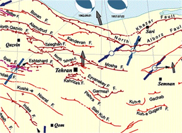
Table 1Characteristics of selected Tehran faults
Fault | Length (km) | Closest distance to the site (km) | |
NorthTehran (NR) | 75 | 11 | 6.9 |
Mosha (M) | 200 | 27 | 7.5 |
Pishva (P) | 34 | 72 | 6.5 |
North Ray (NR) | 17 | 14 | 6.1 |
South Ray (SR) | 18.5 | 12 | 6.2 |
Garmsar (G) | 70 | 58 | 6.9 |
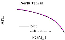
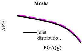
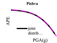
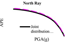
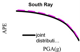
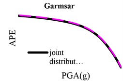
Results of the conventional and proposed methods are shown in Fig. 2 for different faults. In this figure, the solid and dashed lines display hazard curves for the conventional method and the joint-distribution-based approach, respectively. This figure shows how employing statistical variations of leads to more accurate hazard curves. It is seen that, in all cases, the hazard curve of the proposed method is lower than that of the conventional method, even though the difference between these two methods is not identical for different faults as well as within a fault.
To evaluate the effect of the proposed method on hazard curves more precisely, we assess the changes of hazard curves in scenarios with constant annual probability of exceedance (APE) and constant intensity measure. Three values of APE are of interest: 0.01 (the probability of exceedance of 50 % in 50 years), 0.0021 (the probability of exceedance of 10 % in 50 years) and 0.0004 (the probability of exceedance of 2 % in 50 years). PGAs of the conventional and proposed methods are given in Table 2 for the above three APEs. Similarly, APEs are shown in Table 3 for three constant intensity measures, namely, 0.20, 0.35 and 0.50. These tables show that the results of the proposed method are slightly lower than that of the traditional methods. The level of differences is not constant. In order to assess the results more accurately, we computed the percentage of PGA and APE reduction, which are shown in Table 4. According to this Table, in the case of constant APEs, different fault-induced PGAs are decreased 6-17 %, 3-16 % and 1-9 % for APEs equal to 50 %, 10 % and 2 %, respectively. It means that decrease in APEs leads to convergence between the two curves. Thus, hazard curve modification based on distribution has more influences in low APEs. Especially, in the case of serviceability earthquake, the effects of the joint method are significant. In the case of constant intensity measure (PGAs), APEs change between 8 % and 27.2 %. Regarding the order of the APE numbers, the differences are very small. So, we report the results with 4 decimal places. Also in this case, increase in PGAs leads to decrease in percentage of hazard reduction. There is no meaningful relation between faults characteristics and reduction percentage in hazard curves. In order to evaluate the effects of the parameters of the selected distribution for on the hazard curve, we performed the sensitivity analysis of the PSHA in terms of the mean and standard deviation.
Fig. 2Hazard curves for studied faults
a)
b)
c)
d)
e)
f)
Table 2PGAs (g) changes via different methods (in constant APEs)
Fault | PGA ( 0.01) | PGA ( 0.0021) | PGA ( 0.0004) | |||
CA | PA | CA | PA | CA | PA | |
NT | – | – | 0.09 | 0.07 | 0.19 | 0.17 |
M | 0.23 | 0.18 | 0.42 | 0.38 | 0.59 | 0.57 |
P | 0.27 | 0.22 | 0.48 | 0.52 | 0.66 | 0.69 |
NR | 0.18 | 0.17 | 0.42 | 0.40 | 0.66 | 0.65 |
SR | 0.20 | 0.17 | 0.41 | 0.37 | 0.62 | 0.59 |
G | – | – | 0.09 | 0.08 | 0.17 | 0.16 |
CA: Conventional approach, PA: Proposed approach | ||||||
Table 3APEs changes via different methods (in constant PGAs)
Fault | PGA ( 0.01) | PGA ( 0.0021) | PGA ( 0.0004) | |||
CA | PA | CA | PA | CA | PA | |
NT | 0.0003 | 0.0002 | 3.7E-05 | 2.7E-05 | 1.6E-06 | 1.2E-06 |
M | 0.0124 | 0.0091 | 0.0038 | 0.0028 | 0.0010 | 0.0007 |
P | 0.0159 | 0.0235 | 0.0056 | 0.0083 | 0.0017 | 0.0026 |
NR | 0.0090 | 0.0083 | 0.0033 | 0.0030 | 0.0012 | 0.0011 |
SR | 0.0104 | 0.0077 | 0.0034 | 0.0025 | 0.0011 | 0.0008 |
G | 0.0001 | 0.0001 | 3.9E-07 | 2.9E-07 | 1.4E-10 | 1.1E-10 |
CA: Conventional approach, PA: Proposed approach | ||||||
Table 4Hazard reduction percentage via proposed method
Faults | PGA (g) | APE | ||||
Constant APE | Constant PGA | |||||
0.01 | 0.0021 | 0.0004 | 0.2 g | 0.35g | 0.5g | |
NT | 0.06 | 0.03 | 0.01 | 0.084189 | 0.083267 | 0.080044 |
M | – | 0.16 | 0.09 | 0.259857 | 0.256192 | 0.254253 |
P | – | 0.11 | 0.08 | 0.351090 | 0.345390 | 0.340937 |
NR | 0.17 | 0.08 | 0.04 | 0.261914 | 0.263420 | 0.262841 |
SR | 0.16 | 0.08 | 0.04 | 0.260958 | 0.263117 | 0.262680 |
G | – | 0.15 | 0.08 | 0.258325 | 0.256846 | 0.256244 |
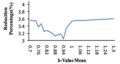
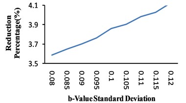
The results are shown in Fig. 3 for the 0.0021. As can be seen from this figure, -value averages have no significant effects on the reduction percentage. But, the increase of standard deviation leads to more reduction in hazard. In this situation, the level of hazard decrease tends to become uniform.
It seems that the level of hazard reduction depends on the -value distribution parameters more than fault characteristics. It is worth mentioning that the distribution parameters are a function of seismicity of the region. In other words, lower seismicity fluctuations and higher numbers of earthquakes make the standard deviation to decrease.
Fig. 3Effects of b-value distribution parameters on hazard curves
a)
b)
5. Discussion
Eq. (14) is a new development of PSHA formulation that considers recurrence law parameters uncertainty. The direct effect of this development is the improvement of the accuracy of computational results. In the previous section, we considered a broad range of examples to evaluate the proposed method. It is expected that the proposed method has similar effects in other situations.
From Fig. 2, it is observed that the beginning and the end of the curve of the proposed method are much lower than that of the conventional method. The slopes of both curves also show a similar behavior. In the middle part of the curves (i.e., for PGAs from 0.3 to 0.55), the curves of the both methods converge.
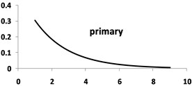
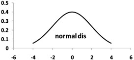
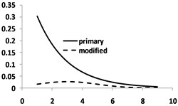
This behavior is due to the correction effects of the normal distribution. According to G-R law, magnitude-frequency distribution in relationship to -value is exponential (see Fig. 4(a)) and -value follows normal distribution (Fig. 4(b)). Thus, the joint distribution of the magnitude and -value is equal to the product of normal and exponential distributions. To illustrate more graphically the effect of the joint PDF, the product of the two PDFs is shown in Fig. 3(c) In the conventional method with fixed , it is assumed that has a uniform distribution. In these circumstances, all values of the magnitude exponential function are scaled with a constant number equal to . Obviously, scaling maintains the shape of the G-R curve. But if residuals change according to the normal distribution, the resulting curve decreases in the beginning and the end and increases in the central part due to the scale factor changes.
Fig. 4Magnitude-frequency distribution modification via normal distribution (numbers are scaled for better illustration): a) Primary exponential distribution; b) Normal distribution; c) Comparing the product of the two distributions with the primary distribution
a)
b)
c)
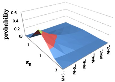
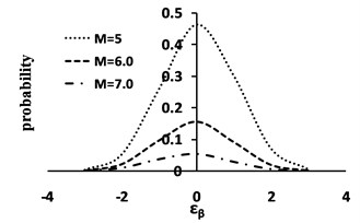
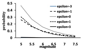
Fig. 5 shows the 3D diagram of the joint PDF (Eq. (13)) and its behavior in the direction of each variable. This figure demonstrates a more intuitive picture of how -value variations will affect the computed hazard. So, Eq. (13) represents an extended formulation of the G-R law that contains parameter uncertainty and can be considered as a probabilistic G-R law. In contrast to the conventional G-R law which is only a function of the magnitude, the proposed probabilistic G-R law has two dimensions, namely, magnitude and .
Fig. 5a) Joint distribution behavior; b) Normal in one direction; c) Exponential in the other
a)
b)
c)
Analogous to the procedures developed to deal with uncertainties in attenuation relationships [28] and the peak-velocity effect [29], inserting the probabilistic G-R law in the triple integral of the conventional PSHA adds new dimension () to it. Although this will slightly increase the computational cost, the accuracy of the hazard curves will improve. While written for PGA, the PSHA equation (i.e. Eq. (14)) also holds if PGA is replaced by virtually any other candidate scalar intensity measure.
6. Conclusion
Hazard curve uncertainty is a key difficulty in PSHA. This uncertainty results from data, models and parameters uncertainties. -value is one of the well-known effective parameters in PSHA. An analytical method of evaluating the seismic hazard uncertainties has the advantage that consistent estimates of hazard can be prepared for various sites. The proposed method provides a novel approach to quantify the parameter uncertainty of -value and express it in a closed-form relation. This relation explicitly exerts regression errors and the corresponding distribution into the analysis. Simplicity, applicability and efficiency of the method are illustrated via the practical examples of faults for different conditions. The results show that the maximum magnitude and the length of the faults as well as its distance to the site have no noticeable effect on the level of hazard curve improvement. The level of improvement varies with distribution standard deviation obtained for -value. This parameter in turn depends on the seismicity of the region.
The proposed method will improve the usefulness and precision of PSHA results. It can be used to test the variability of hazard maps of codes and to evaluate the sufficiency of the original design loads and possible need for upgrading the facility.
References
-
Bommer J. J., Abrahamson N. A. Why do modern probabilistic seismic hazard analyses often lead to increased hazard estimates? Bulletin of the Seismological Society of America, Vol. 96, Issue 6, 2006, p. 1967-1977.
-
Bommer J. J., Scherbaum F., Bungum H., Cotton F., Sabetta F., Abrahamson N. A. On the use of logic trees for ground-motion prediction equations in seismic-hazard analysis. Bulletin of the Seismological Society of America, Vol. 95, Issue 2, 2005, p. 377-389.
-
Gutenberg B., Richter C. Seismicity of the earth and associated phenomena. Princeton University Press, Princeton, New Jersey, 2nd edition, 1954.
-
Gulia L., Meletti C. The influence of b-value estimate in seismic hazard assessment. In First European Conference on Earthquake Engineering and Seismology, 2006.
-
Burroughs S. M., Tebbens S. F. The upper-truncated power law applied to earthquake cumulative frequency-magnitude distributions: Evidence for a time-independent scaling parameter. Bulletin of the Seismological Society of America, Vol. 92, Issue 8, 2002, p. 2983-2993.
-
Wyss M., Stefansson R. Nucleation points of recent mainshocks in southern Iceland, mapped by b-values. Bulletin of the Seismological Society of America, Vol. 96, Issue 2, 2006, p. 599-608.
-
Wiemer S., Wyss M. Mapping spatial variability of the frequency-magnitude distribution of earthquakes. Advances in Geophysics, Vol. 45, 2002, p. 259-302.
-
Johnston A. C., Nava S. J. Recurrence rates and probability estimates for the New Madrid seismic zone. Journal of Geophysical Research: Solid Earth, Vol. 90, Issue B8, 1985, p. 6737-6753.
-
Wiemer S., Katsumata K. Spatial variability of seismicity parameters in aftershock zones. Journal of Geophysical Research: Solid Earth, Vol. 104, Issue B6, 1999, p. 13135-13151.
-
Shi Y., Bolt B. A. The standard error of the magnitude-frequency b-value. Bulletin of the Seismological Society of America, Vol. 72, Issue 5, 1982, p. 1677-1687.
-
Orlecka-Sikora B. Resampling methods in nonparametric seismic hazard estimation. Acta Geophys Pol., Vol. 52, Issue 1, 2004, p. 15-27.
-
Cornell C. A. Engineering seismic risk analysis. Bulletin of the Seismological Society of America, Vol. 58, Issue 5, 1968, p. 1583-1606.
-
Benjamin J. R., Cornell C. A. Probability, statistics, and decision theory for civil engineers. McGraw-Hill, New York, 1970.
-
Abrahamson N. A. Notes on probabilistic seismic hazard analysis – an overview. Rose School, Pavia, Italy, 2006.
-
Krinitzsky E. L. Earthquake probability in engineering – Part 2: Earthquake recurrence and limitations of Gutenberg-Richter b-values for the engineering of critical structures: The third Richard H. Jahns distinguished lecture in engineering geology. Engineering Geology, Vol. 36, Issue 1, 1993, p. 1-52.
-
Lombardi A. M. The maximum likelihood estimator of b-value for mainshocks. Bulletin of the Seismological Society of America, Vol. 93, Issue 5, 2003, p. 2082-2088.
-
Bender B. Maximum likelihood estimation of b values for magnitude grouped data. Bulletin of the Seismological Society of America, Vol. 73, Issue 3, 1983, p. 831-851.
-
Wang Z. Seismic Hazard assessment: issues and alternatives. Pure and Applied Geophysics, Vol. 168, Issue 1-2, 2011, p. 11-25.
-
Lin W. T., Hsieh M. H., Wu Y. C., Huang C. C. Seismic analysis of the condensate storage tank in a nuclear power plant. Journal of Vibroengineering, Vol. 14, Issue 3, 2012, p. 1021-1030.
-
Kijko A., Funk C. W. The assessment of seismic hazards in mines. Journal of the South African Institute of Mining and Metallurgy, Vol. 94, Issue 7, 1994, p. 179-185.
-
Efron B. Bootstrap methods: another look at the jackknife. The Annals of Statistics, Vol. 7, Issue 1, 1979, p. 1-26.
-
United States geological survey website. 2012, http://earthquake.usgs.gov/.
-
Nicknam A., Barkhodari M. A., Jamnani H. H., Hosseini A. Compatible seismogram simulation at near source site using multi-taper spectral analysis approach (MTSA). Journal of Vibroengineering, Vol. 14, Issue 3, 2013, p. 626-638.
-
Sliaupa S. Modeling of the ground motion of the maximum probable earthquake and its impact on buildings, Vilnius city. Journal of Vibroengineering, Vol. 15, Issue 2, 2013, p. 532-543.
-
Ramazi H. R. Attenuation laws of Iranian earthquakes. Proceedings of the Third International Conference on Seismology and Earthquake Engineering, Tehran, Iran, 1999.
-
Ambraseys N. N., Bommer J. J. The attenuation of ground accelerations in Europe. Earthquake Engineering and Structural Dynamics, Vol. 20, Issue 12, 1991, p. 1179-1202.
-
Sarma S. K., Srbulov M. A simplified method for prediction of kinematic soil-foundation interaction effects on peak horizontal acceleration of a rigid foundation. Earthquake Engineering and Structural Dynamics, Vol. 25, Issue 8, 1996, p. 815-836.
-
Moss R. E. S. Reduced uncertainty of ground motion prediction equation through Bayesian variance analysis. Pacific Earthquake Engineering Research Centre, PEER, report, 2009.
-
Tothong P., Cornell C. A., Baker J. W. Explicit directivity-pulse inclusion in probabilistic seismic hazard analysis. Earthquake Spectra, Vol. 23, Issue 4, 2007, p. 867-891.
About this article

The authors would like to appreciate the reviewers and the editor, who have provided valuable comments that significantly improved the original manuscript.
