Abstract
Bearings are used in a wide variety of rotating machineries. Bearing vibration signals are non-stationary signals. According to the non-stationary characteristics of bearing vibration signals, a bearing performance degradation assessment/prediction and fault diagnosis method based on empirical mode decomposition (EMD) and principal component analysis (PCA)-self organizing map (SOM) is proposed in this paper. First, vibration signals are decomposed into a finite number of intrinsic mode functions, after which the EMD energy feature vector, which is composed of all the IMF energy, is obtained. PCA is then introduced to reduce the dimension of feature vectors. After that, the reduced feature vectors are selected as input vectors of the SOM neural network for performance degradation and fault diagnosis. Finally, the degradation trend of bearing is predicted by Elman neural network. The analysis results from bearings with different fault degrees or degradation trend and fault patterns show that the proposed method can assess and predict the degradation of bearing suitably and achieve a fault recognition rate of over 95 % for various bearing fault patterns.
1. Introduction
Bearing is one of the most important elements in a rotary machine. To a great degree, bearing performance influences the performance of the whole machine. To prevent unexpected bearing failure that might cause costly downtime or even casualties, performance degradation assessment/prediction and fault diagnosis has received considerable attention for many years. To prevent unexpected bearing failure, vibration signal analysis based method, which is the most suitable and effective for bearing, has been applied extensively.
A variety of bearing performance degradation assessment/prediction and diagnosis studies have been developed. These studies mainly focus on four aspects: signal analysis, overlap or distance calculation, health index prediction and pattern recognition. To analyze vibration signals and extract features, different techniques such as time domain, frequency domain and time-frequency domain are extensively used. The vibration signals of bearing are non-stationary signals with a large amount of noise, which make the bearing faults very difficult to detect by conventional time domain and frequency domain analysis. Wavelet-based methods have recently been widely used for the assessment and diagnosis of rolling element bearing [1, 2]. However, wavelet transform still has some inevitable deficiencies, including interference terms, border distortion and energy leakage, all of which will generate a large number of small undesirable spikes all over the frequency scales, thus making the results confusing [3]. Empirical mode decomposition (EMD), was then demonstrated to be superior to wavelet analysis in many applications [3-5]. EMD is based on the local characteristic time scales of a signal and could decompose the complicated signal into a number of intrinsic mode functions (IMFs). Frequency components contained in each IMF not only relate to the sampling frequency, but also change with the signal itself. The performance degradation of bearing is always assessed by calculating the overlap or distance between the real-time features and the baseline features in the feature space, and algorithms such as GMM and SOM are always introduced in. Qiu and Lee introduced enhanced and robust prognostic methods for bearing including a wavelet filter based method for fault identification and SOM based method for performance degradation assessment [6, 7]. Howerver, distortion occurs when the high-dimensional data is mapped into low-dimensional data by using SOM. Meanwhile, training a SOM network with high-dimensional data is a time-consuming process. For bearing performance prediction, many time series analysis methods, such as auto regressive and moving average (ARMA) model are widely used, but most of these methods are applicable to predict the performance of linear time-invariant systems whose peroformance features display stationary behavior (without frequent components change over time). Fault diagnosis can be seen as a problem of pattern recognition to which various intelligent methods such as artificial neural network (ANN), hidden Markov model (HMM) and support vector machine have been applied [8]. However, many classification algorithms, such as radial basis function and support vector machine, are unsuitable for performance degradation assessment.
To solve the aforementioned problems, a method that combines EMD, PCA-SOM and Elman neural network is proposed in this paper.
2. Methodology
Performance degradation assessment/prediction and fault diagnosis of bearing based on EMD, PCA-SOM and Elman neural network are shown in Fig. 1. The method is composed of three parts: performance degradation assessment, performance prediction and fault diagnosis. The result of performance degradation assessment is quantitatively indicated by confidence value (CV), following Lee (1996). CV ranges from 0 to 1, which indicates unacceptable and normal performance, respectively over time. Once the CV of a bearing decrease to 0.8, which indicates the occurrence of degradation, the diagnosis algorithm is used to classify bearing faults. For performance degradation assessment, the original vibration signal is decomposed by EMD, and some IMF components are obtained firstly.
Fig. 1Performance assessment/prediction fault diagnosis based on EMD, PCA-SOM and Elman
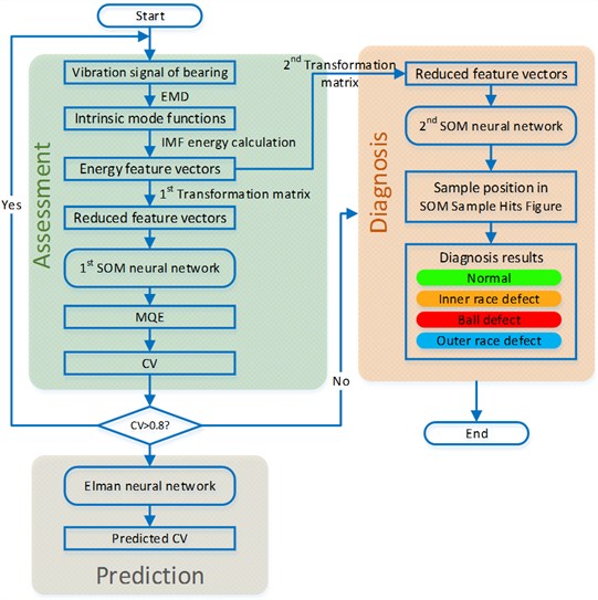
As the IMF energy of different vibration signals illustrate the energy of acceleration vibration signal in different frequency bands and will change when bearing fault occurs, the energy feature vectors are obtained by calculating the energy of each IMF component. PCA is introduced in to reduce the dimension of energy feature vector. Finally, the first SOM neural network, which is trained with normal bearing data, is used to assess the performance degradation of bearing. After performance assessment, an Elman neural network, which is trained by using historical data, is used to predict the CV of the next several cycles [9]. For fault diagnosis, to identify the fault pattern of bearing, another SOM neural network that is trained (labeled) with data of different fault patterns (normal, inner race defect, ball defect, and outer race defect) and served as a fault classifier. The reduced feature vectors are taken as neural network input vectors. By observing the sample position in the SOM figure, the bearing fault pattern can be determined.
2.1. Feature extraction with empirical mode decomposition
The EMD method is developed from the simple assumption that any signal consists of different simple intrinsic modes of oscillations. Each linear or nonlinear mode will have the same number of extrema and zero-crossings. There is only one extremum between successive zero-crossings. Each mode should be independent of the others. In this way, each signal could be decomposed into a number of IMFs, each of which must satisfy the following definition:
Definition 1. In the whole data set, the number of extrema and the number of zero-crossings must either be equal or differ at most by one.
Definition 2. At any point, the mean value of the envelope defined by local maxima and the envelope defined by the local minima is zero.
An IMF represents a simple oscillatory mode compared with the simple harmonic function.
The steps of EMD are as follows.
1) Find out all the maximum points and minimum points of the original signal , and fit fluctuation envelope of the original signal with cubic spline function.
2) Calculate mean value of the fluctuation envelope, denoted by , and make original data sequence minus the mean value to obtain a new data sequence :
3) Judges whether it meets the IMF conditions, if is an IMF, then is the first component of . Otherwise repeat the above two processes until the mean value of is close to zero, then the first IMF component is obtained, it represents the highest frequency components of the signal .
4) Separating the first IMF component from the original signal , and obtain the rest signal without the highest frequency component from original signal:
5) Regard as original signal and repeat the above four processes until the residue function is monotonic function, then other IMF components (1, 2, …, ) can be obtained.
Actually, the process can be stopped by any of the following predetermined criteria: either when the component , or the residue, , becomes so small that it is less than the predetermined value of substantial consequence, or when the residue, , becomes a monotonic function from which no more IMF can be extracted. Even for data with zero mean, the final residue can still be different from zero; for data with a trend, then the final residue should be that trend [10].
With above processes, the original signal can be decomposed as:
Thus, a decomposition of the signal into empirical modes can be achieved, and a residue , which is the mean trend of is also obtained.
While a bearing with different faults is in operation, the corresponding resonance frequency components are produced in the vibration signals, and the energy of the fault vibration signal changes with the frequency distribution. To illustrate this case, the energy of each IMF is calculated.
If IMFs () and a residue are obtained from the vibration signals , the EMD energy feature vectors are calculated as follows:
1) Calculate the total energy of IMFs:
2) Construct a feature vector with the energy as element:
3) For the convenience of PCA and SOM neural network training, the energy feature vectors are normalized as follows:
Then:
2.2. Feature reduction with principal component analysis
PCA is a kind of multivariable analysis method. By using variable transform, we change correlated variables into uncorrelated new variables, which is useful for data analysis [11]. Thus, PCA is widely used for multi-dimension analysis. The general method of PCA is described in Reference [12]. PCA is currently widely used to decrease redundancy and to reduce data to enhance analysis efficiency.
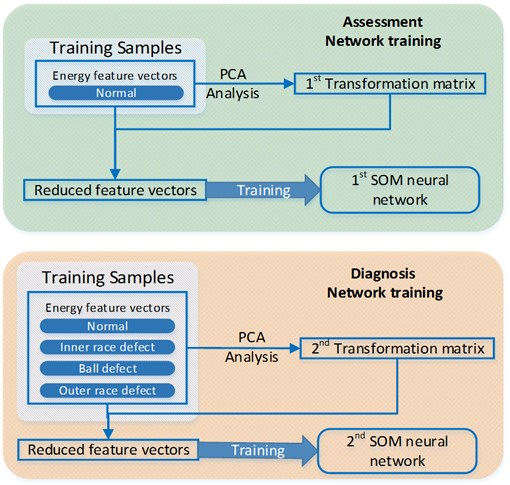
In this paper, the EMD feature vectors are transformed to reduced feature vectors with a transformation matrix. Notably, the transformation matrix in performance degradation assessment and that in fault diagnosis are different matrices. As shown in Fig. 2, the first transformation matrix is used to reduce the dimensions of the feature space, which is composed of the feature vectors of a normal bearing, whereas the other consists of feature vectors of all fault patterns (normal, inner race defect, ball defect, and outer race defect).
Fig. 2PCA analysis and SOM neural network training
2.3. Assessment and diagnosis with SOM neural network
The SOM neural network structure is composed of the input and competitive layers. The input layer is a one-dimensional vector, and the competition level is a two-dimensional planar array [13]. SOM neural network is used to assess the performance degradation and classify the bearing fault pattern in this paper.
For performance degradation assessment, SOM is trained with vibration signals from a normal bearing (see Fig. 2). For each input feature vector, a best match unit (BMU) can be found in the SOM. The distance between the input data feature vector and the weight vector of the BMU, which can be defined as minimum quantization error (MQE) [4], actually indicates how far the input data feature vector deviates from the feature vector of normal bearing. Thus, the degradation trend can be visualized based on the trend of the MQE. As the MQE increases, the extent of degradation becomes more severe. A threshold can be set as the maximum expected MQE, and the degradation extent can be normalized by converting the MQE into CV, in which MQE increases while the CV decreases.
For fault diagnosis, the cluster-then-label method is employed. SOM provides a method by which to represent a multidimensional feature space in a one- or two-dimensional space while preserving the topological properties of the input feature space. In this way, the feature vectors from the same fault pattern can cluster together in the two-dimensional space, which can be observed in SOM sample hits figure. SOM is trained with reduced feature vectors from all fault patterns (see Fig. 2). We then identify the clusters of each input vector. Each cluster is marked with a single color, which enables the prediction of the label of every cluster.
2.4. Prediction with Elman neural network
Elman neural network is a kind of typical dynamic neural network, usually it has four layers: input layer, middle layer (hidden layer), acceptor layer and output layer. The connection of input layer, hidden layer and output layer is similar to the feed-forward network. The cells of input layer only transmit the signals and the cells of output layer have the function of linear weighting. The transfer function of the cells in hidden layer can be linear and non-linear function. The acceptor layer is also called context layer or state layer, which is used for memorizing the previous time step output of hidden layer, so it can be regarded as a one-step time delay operator.
The characteristic of Elman neutral network is that by the delay and storage of acceptor layer, the output of hidden layer connects with the input of hidden layer by itself. This kind of self connection is sensitive to the data of its historical state, the inside feedback network also increases the ability of dynamic information processing so as to serve the purpose of dynamic modeling [14]. With these characteristic, Elman neural network can be used to predict the CV generated by the SOM neural network.
An Elman neural network which is trained with the historical CV is selected to predict the CV synchronously, the data flow diagram is shown in Fig. 1. The predicted CV over time can be used to extrapolate the performance of bearing in the future. Using the last ( ()) values to predict the future () values is called -step prediction, it is desirable that adjacent samples as sliding window, and samples are mapped to values, as is shown in Fig. 3 and Table 1.
Fig. 3M-step prediction
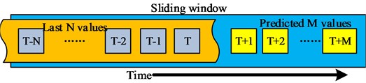
Table 1Inputs and outputs of M-step prediction
inputs | outputs |
, , ..., | , , ..., |
, , ..., | , , ..., |
... | ... |
, , ..., | , , ..., |
3. Experiment results
Two experiment were conducted to illustrate the effectiveness of the presented method. The first experiment mainly focus on the validation of performance degradation assessment and fualt diagnosis while the other experiment is used to validate the effectiveness of performance degradation assessment and prediction.
3.1. Experiment 1: performance assessment and fault diagnosis
The data used in the application experiment come from the bearing data center, which provides access to the ball bearing test data for normal and faulty bearings. In the experiment, three common types of bearing fault were set: inner race defect, ball defect, and outer race defect. To verify the assessment method, single-point faults were introduced to the test bearings using electro-discharge machining with fault diameters of 7, 14, and 21 mils (1 mil0.01 inches). The motor speed is 1750 r/min, and the sampling rate is 120 KHz.
For performance degradation assessment, 100 feature vectors extracted form 100 K vibration signal data were used to train the first SOM neural network, and 80 sets of data were used to validate the algorithm, as shown in Table 2. Notably, one EMD energy feature vector was extracted from every 1000 samples of vibration signal.
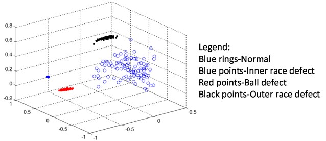
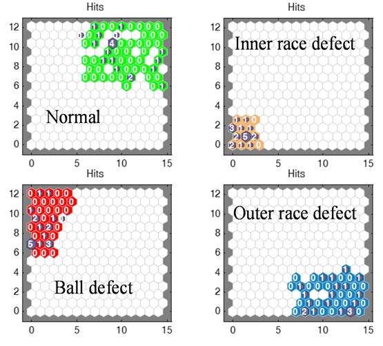
For fault diagnosis, 400 feature vectors, consisting of 100 feature vectors of normal bearing and 300 feature vectors of fault bearing (including inner race defect, ball defect, and outer race defect), as shown in Fig. 4, were used to train the 2nd SOM neural network. After SOM neural network training and clustering, each cluster was marked with a single color (normal: green, inner race defect: yellow, ball defect: red, outer race defect: blue), as shown in Fig. 5. After that, 80 sets of data were used to test the SOM neural network for fault diagnosis (see Table 2).
Table 2Test feature vectors
Test feature vectors for performance degradation assessment | ||||
Pattern | Normal | 7 mils fault | 14 mils fault | 21 mils fault |
Sample size | 20 feature vectors | 20 feature vectors | 20 feature vectors | 20 feature vectors |
No. | 1-20 | 21-40 | 41-60 | 61-80 |
Test feature vectors for fault diagnosis | ||||
Pattern | Normal | Inner race defect | Ball defect | Out race defect |
Sample size | 20 feature vectors | 20 feature vectors | 20 feature vectors | 20 feature vectors |
Fig. 4Feature vectors of bearings (after PCA)
The results of performance degradation assessment of bearings are shown in Fig. 6. The CVs of the first 20 samples, collected from the vibration signals of normal bearing, are significantly higher than 0.8, the predetermined failure threshold, which indicates stable performance. However, other CVs are below the threshold, and CVs decrease when fault diameters increase. These test results indicate that the CV can reflect the performance degradation of bearing well.
Fig. 5SOM samples with training data sets
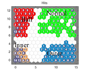
Fig. 6CV of different bearings
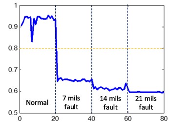
Fig. 7 shows the results of fault diagnosis. The first figure is that of a test with vibration signals of normal bearing, where the green area represents normal states, which are labeled using training samples. In this test, 19 test data sets fell in the green area, and one sample fell out of the area. The second figure is that of a test with vibration signals of bearing with inner race defect. All 20 test data sets fell in the yellow area. The third figure is that of a test with vibration signals of bearing with ball defect, and one sample fell out of the red area. The fourth figure is that of a test with signals from bearings with outer race defect, and all the test data sets fell within the labeled blue area. Thus, two samples out of 80 exhibited misjudgement of fault diagnosis, resulting in a corresponding accuracy of 97.5 %.
Fig. 7SOM sample hits
3.2. Experiment 2: Performance assessment and prediction
The data in this test was generated by the NSF I/UCR Center for Intelligent Maintenance Systems (IMS-www.imscenter.net) with support from Rexnord Corp. in Milwaukee, WI. In the expriment, the rotation speed was kept constant at 2000 RPM by an AC motor coupled to the shaft via rub belts. A radial load of 6000 lbs is applied onto the shaft and bearing by a spring mechanism. The bearing is force lubricated. All failures occurred after exceeding designed life time of the bearing which is more than 100 million revolutions. 1-second vibration signal snapshots were recorded every 100 minutes, and the sample rate is 20 KHz.
Fig. 8Feature vectors of bearing (test-to-failure experiment)
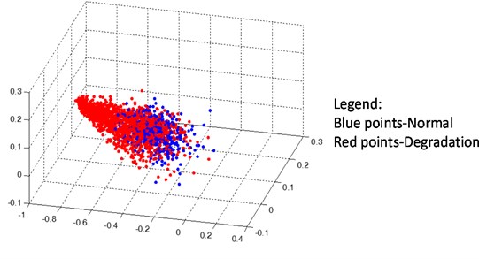
To train the SOM neural network, 501 feature vectors are extracted from 501760 vibration signal data (one EMD energy feature vector is extracted from 1000 samples of vibration signal). Meanwhile, 1005 feature vectors are extracted from 1005280 vibration data to validate the assessment and prediction algorithm. All the feature vectors are processed by PCA before SOM training and performance degradation assessment/prediction. The PCA-processed feature vectors are shown in Fig. 8.
Fig. 9Performance prediction of bearing, (blue curve – current CV, Red curve – predicted CV)
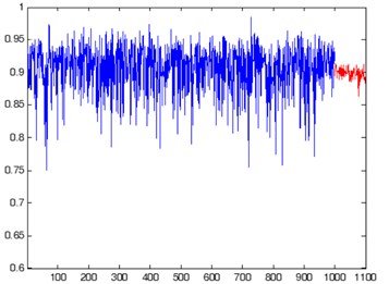
a) 1000
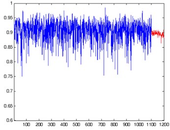
b) 1100
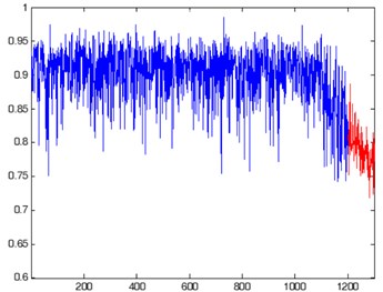
c) 1200
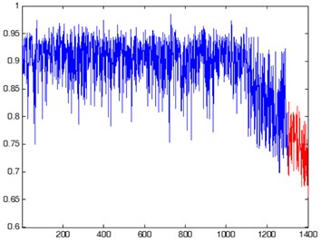
d) 1300
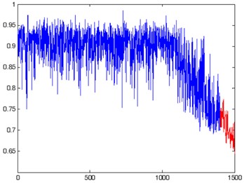
e) 1400
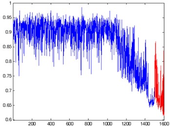
f) 1500
By using the method presented above, CV is obtained from the trained SOM neural network. Then, Elman neural network is trained to predict the CV of next 100 values from value 1001. Considering precision and synchronization of the prediction, the width of the slide window is 300, and the prediction length is 100 steps. Let variable be the current time, the future 100 values () of CV are predicted by using the last 200 values (). It is desirable that 300 adjacent CVs as sliding window, and 200 values are mapped to 100 values, and it keeps CV calculation and prediction synchronous.
The prediction results is shown in Fig. 9. Due to space limitation, six graphics ( 1000, 1100, 1200, 1300, 1400, 1500) of the results are shown in this paper. The results shows that Elman neural network can predict the degradation trend of bearing, based on the performance assessment of bearing.
4. Conclusion
This work presents a method for performance degradation assessment/prediction and fault diagnosis of bearing by using EMD and PCA-SOM. The advantage of the proposed method lies in the efficient synergy between the well-known advantages of SOM unsupervised learning and the feature-extraction tools based on EMD, which enable the discovery of relationships between fault-related features. Moreover, PCA is introduced to reduce the dimension of feature vectors, thus making the assessment and diagnosis more accurate. Finally, Elman neural network is used to predict the degradation trend of bearing, which is benificial to preventative maintenance. Two experiments were conducted to demonstrate the feasibility and effectiveness of the proposed approach.
References
-
Pan Y., Chen J., Li X. Bearing performance degradation assessment based on lifting wavelet packet decomposition and fuzzy c-means. Mechanical Systems and Signal Processing, Vol. 24, Issue 2, 2010, p. 559-566.
-
Wang D. Y., Zhang W. Z., Zhang J. G. Fault bearing identification based on wavelet packet transform technique and artificial neural network. International Conference on System Science, Engineering Design and Manufacturing Informatization, 2010, p. 11-14.
-
Cheng G., Cheng Y.-L., Shen L.-H, et al. Gear fault identification based on Hilbert-Huang transform and SOM neural network. Journal of the International Measurement Confederation, Vol. 46, Issue 3, 2013, p. 1137-1146.
-
Yu Y., Dejie Yu, JunshengC. A roller bearing fault diagnosis method based on EMD energy entropy and ANN. Journal of Sound and Vibration, Vol. 294, Issue 1-2, 2006, p. 269-277.
-
Su W., Wang F., Zhu H., Zhang Z., Guo Z. Rolling element bearing faults diagnosis based on optimal Morlet wavelet filter and autocorrelation enhancement. Mechanical Systems and Signal Processing, Vol. 24, 2010, p. 1458-1472.
-
Qiu H., Lee J., Lin J., et al. Robust performance degradation assessment methods for enhanced rolling element bearing prognostics. Advanced Engineering Informatics, Vol. 17, Issue 3-4, 2003, p. 127-140.
-
Shi S., Zhang L., LiangW. Condition monitoring and fault diagnosis of rolling element bearings based on wavelet energy entropy and SOM. Proceedings of International Conference on Quality, Reliability, Risk, Maintenance, and Safety Engineering, 2012, p. 651-655.
-
Hu Q., He Z., Zhang Z., Zi Y. Fault diagnosis of rotating machinery based on improved wavelet package transform and SVMs ensemble. Mechanical Systems and Signal Processing, Vol. 21, 2007, p. 688-705.
-
Liao L., Lee J. Design of a reconfigurable prognostics platform for machine tools. Expert Systems with Applications, Vol. 37, Issue 1, 2010, p. 240-252.
-
Huang N. E., Shen Z., Long S. R., et al. The empirical mode decomposition and the Hilbert spectrum for nonlinear and non-stationary time series analysis. Proceedings of the Royal Society of London. Series A: Mathematical, Physical and Engineering Sciences, Vol. 454, Issue 1971, 1998, p. 903-995.
-
Liao W., Wang H. Fault diagnosis for power unit based on wavelet packet PCA-SVM. Proceedings of the 29th Chinese Control Conference, 2010, p. 3851-3855.
-
Jolliffe I. T. Principal component analysis. Springer-Verlag New York, 1986.
-
Hu J., Zhang L., Liang W. Degradation assessment of bearing fault using SOM network. 7th International Conference on Natural Computation, 2011, p. 561-565.
-
Li P., Li Y., Xiong Q., et al. Application of a hybrid quantized Elman neural network in short-term load forecasting. International Journal of Electrical Power & Energy Systems, Vol. 55, 2014, p. 749-759.
About this article

This research is supported by the National Natural Science Foundation of China (Grant No. 61074083, 50705005, and 51105019), as well as the Technology Foundation Program of National Defense (Grant No. Z132013B002).
