The flutter of a two-dimensional lifting surface with cubic nonlinearities in a supersonic flow field

1. Introduction

In recent years, many problems concerning the 2-degree-of-freedom (2-DOF) aeroelatstic system with cubic nonlinearity have been successfully studied using the center manifold theory and the normal form method [1-3]. There exist many potential sources of nonlinearities, which can have significant effect on an aeroelastic response. The nonlinearities of the aeroelastic system can be structural [4-5] or aerodynamic [6].

Breitbach [4] presented a detailed review of some possible structural nonlinearities and their effect on aeroelastically induced vibrations. Raghothama and Narayanan [7] investigated periodic oscillations and bifurcations of a two-dimensional airfoil in plunge and pitch motions with cubic pitch stiffness in incompressible flow. Shahrzad and Mahzoon [8] studied the limit cycle oscillation (LCO) flutter of a two-dimensional wing with nonlinear pitch stiffness. Liu, Wong and Lee [9] adopted a point transformation technique to study the nonlinear behavior of a two-dimensional aeroelastic system with freeplay models. Zhao and Zhang [10] investigated the LCO flutter and chaotic motion of a 2-DOF airfoil system with a combination of freeplay and cubic nonlinearities. The Krylov-Bogoliubov-Mitropolsky (KBM) method was used by Yang [11] to study the LCOs of an airfoil with the freeplay nonlinearity. Kim and Lee [12] analyzed the dynamic behavior of a flexible airfoil with the freeplay nonlinearity. Price et al. [13] discovered the LCOs at flow speeds below the linear flutter boundary in a system with a hard pitch spring. Abbas et al. [14] investigated the flutter and post-flutter of a two-dimensional double-wedge lifting surface. The behavior of bifurcation point and the influence of the system parameters on the stability and amplitudes of the LCO flutter were analyzed in references [15-16]. The relation between frequency and airfoil parameters was obtained by means of the harmonic balance method in reference [17].

In this paper, an effective analysis method to the problem of flutter of a two-dimensional airfoil with cubic structural and aerodynamic nonlinearities is proposed. This analysis method enables one to make a parametric study. Firstly, the normal form and universal unfolding are deduced by means of the maple program and the bifurcation theory. Secondly, super- and sub-critical Hopf bifurcations are analyzed. Finally, numerical examples and simulations are given to show the efficiency of this analysis method. Moreover, the influence of the structural and aerodynamic parameters, representations $B$, $M$, and $\gamma$, on the airfoil safety is studied.

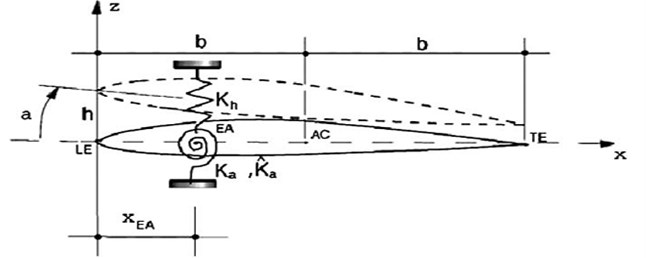
Fig. 1Airfoil section

2. Nonlinear model of a two-dimensional lifting surface

Consider a two-dimensional lifting surface featuring plunging and twisting degrees of freedom, elastically constrained by a linear translational spring and nonlinear torsional spring, as shown in Fig. 1, exposed to a supersonic flow field. The equations of motion of the lifting surface are [18]:

where $h$ is the plunging displacement (positive downward), $\alpha$ the twist angle about the pitch axis (positive nose up), the primes denote differentiation with respect to time $t$, $m$ the structural mass per unit span, $S_{\alpha }$ the static unbalance about the elastic axis, $I_{\alpha }$ the mass moment of inertia about the elastic axis of the airfoil, ${\mathrm{c}}_h$ and ${\mathrm{c}}_{\mathrm{\alpha }}$ are linear plunging and pitching viscous damping coefficients, while $K_h$ is the plunging stiffness coefficient. And ${\stackrel{-}{M}}_{\alpha }$ represents the overall restoring moment that is connected to the pitch angle by:

where $K_{\mathrm{\alpha }}$ and ${\widehat{K}}_{\alpha }$ are the linear and nonlinear pitching stiffness coefficients, respectively. The tracer ${\delta }_S$ that identifies this type of nonlinearities can take the value 1 or 0 depending on whether the nonlinearity is accounted for or discarded, respectively. In addition, the expressions of the aerodynamic lift and moment are:

herein, $b$ is the half-chord length of the airfoil, $x_{EA}=b{x}_0$ is streamwise position of the pitch axis measured from the leading edge, $U_{\infty }$, ${\rho }_{\infty }$ and $M_{\mathrm{\infty }}$ are the air speed, the air density, and the flight Mach number of the disturbed flow, respectively. $\lambda$ and $\gamma$ are correction aerodynamic factor and the isentropic gas coefficient, respectively.

Upon denoting $x_1=h/b$, $x_2=\alpha$, and the dimensionless time $\tau =U_{\infty }t/b$, Eq. (1) can be written as:

where the coefficients can be found in Appendix, and the dots denote $d/d\tau$.

3. The stability and bifurcation analysis of system (4)

3.2. Normal form, universal unfolding and Hopf bifurcation

Choosing the following dimensionless values of parameters as [18]: $\mu =\text{100}$, ${\chi }_{\alpha }=\text{0.25}$, $x_0=\text{0.5}$, $r_{\alpha }=\text{0.5}$, $\varpi =\text{1.2}$, ${\zeta }_{\alpha }={\zeta }_h=\text{0}$ and $\lambda =\text{1}$, Eq. (4) can be rewritten as:

10

$\left(\begin{array}{l}{\dot{x}}_1\\ {\dot{x}}_2\\ {\dot{x}}_3\\ {\dot{x}}_4\end{array}\right)=A\left(\begin{array}{l}{x}_1\\ x_2\\ x_3\\ x_4\end{array}\right)+f{x}_2^3,$

where:

$A=\left(\begin{array}{cccc}0& 0& 1& 0\\ 0& 0& 0& 1\\ \frac{-1.92}{V^2}& \frac{50M-V^2}{150M{V}^2}& \frac{-1}{150M}& \frac{1}{900M}\\ \frac{1.92}{V^2}& \frac{-100M-V^2}{75M{V}^2}& \frac{-1}{75M}& \frac{-1.1}{45M}\end{array}\right),f=\left(\begin{array}{c}0\\ 0\\ \frac{-M(1+\gamma )}{1800}\\ \frac{-M(1+\gamma )}{900}\end{array}\right)+\left(\begin{array}{c}0\\ 0\\ \frac{B}{3V^2}\\ \frac{-B}{0.75V^2}\end{array}\right).$

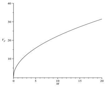
Substituting the above dimensionless values of parameters and the Eq. (7) into the first formula of (9), the speed on the flutter instability boundary is:

11

$V_F=\sqrt{\frac{7.850112004\times 10^{11}{M}^2}{-3.90656\times 10^8+1.5859199\times 10^{10}M}}.$

The relation of the flutter speed $V_F$ and flight Mach number $M$ is depicted in Fig. 2. The figure reveals that the increase of flight Mach number can result in the increase of the flutter safety.

Fig. 2The flutter speed VF vs. flight Mach number M

In the following, we assume $O$ is a bifurcation point, i.e. the conditions (9) hold. Substituting $V=V_F$ into Eq. (10), we get:

12

$\left(\begin{array}{l}{\dot{x}}_1\\ {\dot{x}}_2\\ {\dot{x}}_3\\ {\dot{x}}_4\end{array}\right)=\stackrel{-}{A}\left(\begin{array}{l}{x}_1\\ x_2\\ x_3\\ x_4\end{array}\right)+\stackrel{-}{f}{x}_2^3,$

where:

$\stackrel{-}{A}=\left(\begin{array}{cccc}0& 0& 1& 0\\ 0& 0& 0& 1\\ \frac{-1.92}{V_F^2}& \frac{50M-V_F^2}{150M{V}_F^2}& \frac{-1}{150M}& \frac{1}{900M}\\ \frac{1.92}{V_F^2}& \frac{-100M-V_F^2}{75M{V}_F^2}& \frac{-1}{75M}& \frac{-1.1}{45M}\end{array}\right),\stackrel{-}{f}=\left(\begin{array}{c}0\\ 0\\ \frac{-M(1+\gamma )}{1800}\\ \frac{-M(1+\gamma )}{900}\end{array}\right)+\left(\begin{array}{c}0\\ 0\\ \frac{B}{3{V_F}^2}\\ \frac{-B}{0.75{V_F}^2}\end{array}\right).$

For Eq. (12), there is a coordinate transformation $x=Py\text{,}$$x=(x_1,x_2,x_3,x_4{)}^T\text{,}$$y=(y_1,y_2,y_3,y_4{)}^T$ so that:

13

$\dot{y}=Jy+g{\left(\sum _{j=1}^4{P}_{2j}{y}_j\right)}^3,$

where $J=P^{-1}\stackrel{-}{A}P=\left(\begin{array}{l}0-\omega 00\\ \omega 000\\ 00-\alpha -\beta \\ 00\beta -\alpha \end{array}\right)$, $\pm \mathrm{i}\omega$ and $-\alpha \pm \mathrm{i}\beta$ are the eigenvalues of the matrix $\stackrel{-}{A}$, and $g=(g_1,g_2,g_3,g_4{)}^T=P^{-1}\stackrel{-}{f}$.

Using the Maple program in reference [19], the normal form of Eq. (13) is calculated as:

14

$\left(\begin{array}{l}{\dot{z}}_1\\ {\dot{z}}_2\end{array}\right)=\left(\begin{array}{ll}0& -\omega \\ \omega & 0\end{array}\right)\left(\begin{array}{l}{z}_1\\ z_2\end{array}\right)+(z_1^2+z_2^2)\left\{\left.{\delta }_1\left(\begin{array}{l}{z}_1\\ z_2\end{array}\right)+{\delta }_2\left(\begin{array}{l}-z_2\\ z_1\end{array}\right)\right\}\right.,$

where:

15

${\delta }_1=\frac{3}{8}\left(g_1{P}_{21}{P}_{22}^2+g_1{P}_{21}^3+g_2{P}_{22}{P}_{21}^2+g_2{P}_{22}^3\right),$
${\delta }_2=\frac{-3}{8}(g_1{P}_{22}{P}_{21}^2+g_1{P}_{22}^3-g_2{P}_{21}{P}_{22}^2-g_2{P}_{21}^3).$

The coordinate transformation $y=Tz$ is omitted here (for details, see the Maple program in reference [19]).

If ${\delta }_1\ne 0$, the universal unfolding of Eq. (14) can be written as [20]:

16

$\left(\begin{array}{l}{\dot{z}}_1\\ {\dot{z}}_2\end{array}\right)=\left(\begin{array}{ll}\nu & -\omega \\ \omega & \nu \end{array}\right)\left(\begin{array}{l}{z}_1\\ z_2\end{array}\right)+(z_1^2+z_2^2)\left\{\left.{\delta }_1\left(\begin{array}{l}{z}_1\\ z_2\end{array}\right)+{\delta }_2\left(\begin{array}{l}-z_2\\ z_1\end{array}\right)\right\}\right..$

Because Eq. (16) is the universal unfolding of Eq. (14), Eq. (16) bears all the dynamic behavior of any small perturbed system of Eq. (14) in the vicinity of $z={\left(z_1,z_2\right)}^T=0$. Furthermore, using the transformations $P$ and $T$, we can obtain all the dynamic behavior of any small perturbed system of Eq. (12) in the vicinity of $O$.

Let $z_1=r\mathrm{c}\mathrm{o}\mathrm{s}\theta$ and $z_2=r\mathrm{s}\mathrm{i}\mathrm{n}\theta$, then the polar coordinate form of Eq. (16) is:

17

$\left\{\begin{array}{l}\dot{r}=r(\nu +{\delta }_1{r}^2),\\ \dot{\theta }=\omega +{\delta }_2{r}^2.\end{array}\right.$

Now we derive the expression of the unfolding parameter $\nu$ in Eq. (17).

Consider one of the perturbed systems of Eq. (12) as follows. Without loss of generality, using the parameter transformations $V=V_F+\eta$ and the state variable transformation $x=Py$, one may transform Eq. (12) into a new system as follows:

18

$\dot{y}=P^{-1}{\stackrel{-}{A}}_{\eta }Py+P^{-1}{\stackrel{-}{f}}_{\eta }(\sum _{j=1}^4{P}_{2j}{y}_j{)}^3,$

where:

${\stackrel{-}{A}}_{\eta }=\left(\begin{array}{cccc}0& 0& 1& 0\\ 0& 0& 0& 1\\ \frac{-1.92}{{\left(V_F+\eta \right)}^2}& \frac{50M-{\left(V_F+\eta \right)}^2}{150M{\left(V_F+\eta \right)}^2}& \frac{-1}{150M}& \frac{1}{900M}\\ \frac{1.92}{{\left(V_F+\eta \right)}^2}& \frac{-100M-{\left(V_F+\eta \right)}^2}{75M{\left(V_F+\eta \right)}^2}& \frac{-1}{75M}& \frac{-1.1}{45M}\end{array}\right),$

${\stackrel{-}{f}}_{\eta }=\left(\begin{array}{c}0\\ 0\\ \frac{-M(1+\gamma )}{1800}\\ \frac{-M(1+\gamma )}{900}\end{array}\right)+\left(\begin{array}{c}0\\ 0\\ \frac{B}{3{\left(V_F+\eta \right)}^2}\\ \frac{-B}{0.75{\left(V_F+\eta \right)}^2}\end{array}\right).$

Let $L=(L_1,L_2,L_3,L_4{)}^T=P^{-1}{\stackrel{-}{A}}_{\eta }Py$. According to reference [21], in Eq. (17) the unfolding parameter $\nu =\frac{1}{2}\eta \times {\left(\frac{{\partial }^2{L}_1}{\partial y_1\partial \eta }+\frac{{\partial }^2{L}_2}{\partial y_2\partial \eta }\right)}_{y_1=y_2=\eta =0}$. We can obtain the conclusions for Eqs. (16)-(18) as follows:

Case 1: ${\delta }_1<\text{0}$.

If $\nu <\text{0}$, (0,0) is a stable focus of Eq. (16), so (0,0,0,0) is also a stable focus of Eq. (18); if $\nu =\text{0}$, because the solutions of Eq. (17), $r^2=-1/2({\delta }_{1}t+c)$, are attracted to zero when $t\to +\mathrm{\infty }$, (0,0,0,0) is an asymptotically stable, but non-hyperbolic equilibrium point of Eq. (18); if $\nu >\text{0}$, for Eq. (16), (0,0) is an unstable focus and there is a stable LCO , $z_1^2+z_2^2=-v/{\delta }_1$, so for Eq. (18) (0,0,0,0) is an unstable focus and there is a stable LCO as well. Supercritical Hopf bifurcation takes place in this case. In practice, because the amplitude of the LCO builds up from zero gradually as $\nu$ increases, it doesn’t bring immediately failure of the structure. So the flutter instability in this case is benign.

Case 2: ${\delta }_1>\text{0}$.

For Eq. (18), if $\nu <\text{0}$, (0,0,0,0) is a local stable focus, and there is an unstable LCO; if $\nu =\text{0}$, (0,0,0,0) is an unstable non-hyperbolic equilibrium point; if $\nu >0$, (0,0,0,0) is an unstable focus. Subcritical Hopf bifurcation occurs in this case. In practice, when $\nu >\text{0}$, the response with any small initial conditions will move away from the trivial point immediately and the flutter is violent. So the flutter instability in this case is catastrophic.

4. The effect of the structural and aerodynamic parameters on character of the flutter instability

One concludes that the sign of ${\delta }_1$ decides the type of Hopf bifurcation or the character of flutter instability, i.e. benign or catastrophic. ${\delta }_1$ vs. $M$ as a function of the normalized nonlinear stiffness coefficient $B$ when $\gamma =\text{1.4}$ are shown in Fig. 3 (curves are drawn pointwisely by using the first formula of Eq. (15)).

Fig. 3The relations of δ1 and flight Mach number M as a function of the structural nonlinearity B

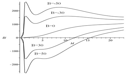
The Fig. 3 indicates that the aerodynamic nonlinearity, representation $M$, and the structural nonlinearity, representation $B$, can affect the sign of ${\delta }_1$.

For $B=-\text{50}$, $-\text{30}$ and $\text{0}$, the whole curves ${\delta }_1-M$ lie above the $M$ axis. So the flutter takes place always as a subcritical Hopf bifurcation for any value of $M$, and the flutter instability is catastrophic. For $B=\text{30}$ and 50, the curves ${\delta }_1-M$ intersect the $M$ axis at the critical values. We define the critical value as $M_c$, at where the sign of ${\delta }_1$ changes from negative to positive. This implies that with the increase of the flight Mach number $M$, the flutter instability changes from benign to catastrophic at last. In other respect, the increase of hard structural nonlinearity ($B>0$) results in the increase of $M_c$ and the flight safety, and for hard structural nonlinearity the decrease of flight Mach number $M$ can increase the flight safety as well.

5. Examples, numerical simulations, and the effect of the parameters on character of the flutter instability

In the following, two cases with the flight Mach number $M=\text{4}$ and $M=\text{10}$ are considered and the flutter speeds are solved from Eq. (11) as $V_{1F}=\text{14.11460254}$ for $M=\text{4,}$ and $V_{2F}=\text{22.27577602}$ for $M=\text{10}$, respectively.

Take $M=\text{4}$ for example. In this case, the parameters in Eq. (16) were determined as:

Fig. 4The relation of δ1, B and γ for M=4

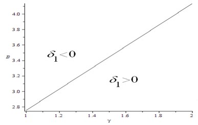
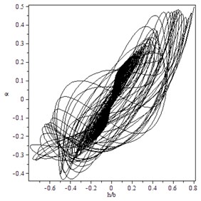
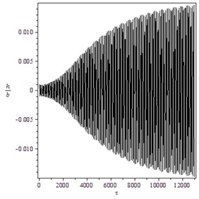
Fig. 5Supercritical Hopf bifurcation for γ=1.4, B=100, M=4: a) trajectory starting from x0T=(0.5,0.28,0,0) converges to O for V=14, b) the transient time history of h/b for V=14.3 and x0T=(0.0001,0.0001,0,0), c) the transient time history of α for V=14.3 and x0T=(0.0001,0.0001,0,0), d) trajectory starting from x0T=(0.5,0.28,0,0) converges to a LCO for V=14.3

a)

b)

c)

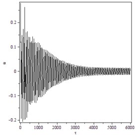
d)

The relation of ${\delta }_1$, $B$ and $\gamma$ is depicted in Fig. 4. The character of flutter instability is benign above the slope line, but it is catastrophic below the slope line. The decrease of isentropic gas coefficient $\gamma$ results in the increase of the flight safety, and the increase of hard structural nonlinearity ($B>\text{0}$) also does.

Fig. 6Subcritical Hopf bifurcation for γ=1.4, B=2.5, M=4: a) trajectory starting from x0T=(0.04,0.0001,0,0) converges to a LCO immediately for V=14, b) trajectory starting from x0T=(0.0002,0.00015,0,0) converges to a LCO for V=14.3

a)

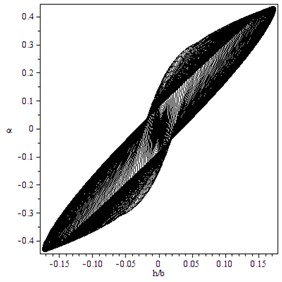
b)

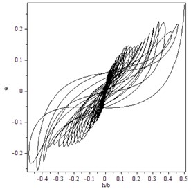
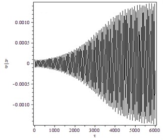
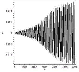
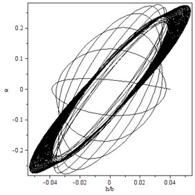
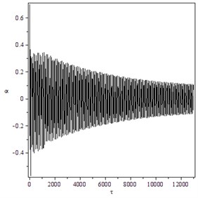
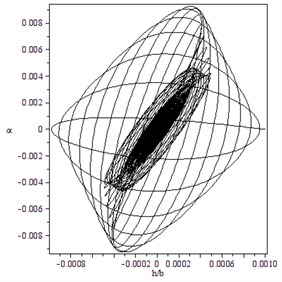
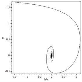
Fig. 7Supercritical Hopf bifurcation for γ=1.4, B=21, M=10: a) trajectory starting from x0T=(0.8,0.5,0,0) converges to O for V=22.1, b) the transient time history of h/b for V=22.5 and x0T=(0.001,0.005,0,0), c) the transient time history of α for V=22.5 and x0T=(0.8,0.7,0,0)

a)

b)

c)

To verify these theoretical results, numerical simulations using the Runge-Kutta algorithm to the Eq. (10) for $M=\text{4}$ were carried out. Notice that $x_1=h/b$, $x_2=\alpha$. When $B=\text{100}$ and $\gamma =\text{1.4}$, ${\delta }_1<\text{0}$. Supercritical Hopf bifurcation occurs, as shown in Fig. 5. Because the amplitude of the LCO is small no matter the initial distance is small or large, the flutter instability is benign. When $B=\text{2.5}$ and $\gamma =\text{1.4}$, ${\delta }_1>\text{0}$. Subcritical Hopf bifurcation occurs, as shown in Fig. 6. The amplitudes of the two LCOs are large, so the flutter instability yields catastrophic failure of the structure.

For the case with the flight Mach number $M=\text{10}$, the flutter speed $V_{2F}=\text{22.27577602}$, ${\delta }_1=\text{27.18679908}+\text{27.18679908}\gamma -\text{3.159223268}B\text{,}$${\delta }_2=\text{51.27974352}+\text{51.27974352}\gamma -\text{5.056781381}B$, and $\nu =\text{0.00227926149}\eta$. The relation of ${\delta }_1$, $B$ and $\gamma$ is similar to what is depicted in Fig. 4. Numerical simulations for the Eq. (10) when $M=\text{10}$ were carried out. When $B=\text{21}$ and $\gamma =\text{1.4}$, ${\delta }_1<\text{0}$, Fig. 7 indicates that the bifurcation is supercritical and the flutter instability is benign. Whilst when $B=-\text{10}$ and $\gamma =\text{1.4,}$${\delta }_1>\text{0}$ Fig. 8 indicates that the subcritical Hopf bifurcation takes place and the flutter instability is catastrophic.

Fig. 8Subcritical Hopf bifurcation for γ=1.4, B=-10, M= 10: a) trajectory starting from x0T=(0.001,0,0,0) converges to O for V=22.1, b) trajectory starting from x0T=(0.00002,0.00001,0,0) moves away from O immediately for V=22.5

a)

b)

6. Conclusions

This paper deals with the flutter of a two-dimensional lifting surfaces in a supersonic flow field. This Eq. (4) undergoes only Hopf bifurcations in the neighborhood of the trivial equilibrium point if this system bifurcates at this point. The normal form and universal unfolding are calculated by using the maple program and the bifurcation theory. The supercritical Hopf bifurcation is benign, because it brings less flutter to the airfoil. Comparably the subcritical Hopf bifurcation is catastrophic, because it renders a harmful violent flutter of the airfoil.

In addition, we study the influence of the structural and aerodynamic parameters, representations $B\text{,}$$M$ and $\gamma \text{,}$ on the character of flutter instability. The influence of these parameters can be described as follows:

1) The soft structural nonlinearities ($B<\text{0}$) yield failure of the structure (i.e. catastrophic flutter), and yet the hard structural nonlinearities ($B>\text{0}$) perhaps not.

2) The increase of hard structural nonlinearity results in the increase of the airfoil safety, and for hard structural nonlinearity the decrease of the flight Mach number $M$ and isentropic gas coefficient $\gamma$ also do.