Fault diagnosis of rotating machinery based on noise reduction using empirical mode decomposition and singular value decomposition

1. Introduction

Rotary machines are one of the most and frequency used equipments in modern industry. For a rotating machine, one common cause of its performance deterioration is bearing failure that will cause fatal machine breakdowns or disastrous accidents [1]. Therefore, there is need to propose a method to effectively diagnose bearing faults in time to reduce mechanical unscheduled downtime. To this end, a great many of effective fault diagnosis methods have been proposed for fault diagnosis of rotating machinery, and most of them are based on vibration signal analysis [1-3].

Feature extraction using a signal processing tool is an important stage of an effective fault diagnosis method. As we all know, the collected vibration signal disturbed by noise is nonlinear and unsteady. Therefore, the traditional signal processing methods may not effectively extract appropriate features for mechanical fault diagnosis [3]. In 1998, the EMD algorithm, a new time-frequency analysis method, was proposed to process complicated signals by Huang et al. [4]. The overlapping in both time and frequency components of a complicated signal can be revealed by these decomposed IMFs which have clear physical meanings [5]. As EMD can deal with nonlinear and non-stationary data sets, so it has a great number of applications in fault diagnosis of rotating machinery. Du and Yang [6] combined EMD and envelope analysis to highlight the CDFs to realize the fault diagnosis of ball bearings. Their experiment with two kinds of vibration signals under normal and faulty bearing condition testified that EMD is more superior to discrete wavelet algorithm in mechanical fault diagnosis. In [7], EMD and autoregressive (AR) model were employed to extract features for the fault diagnosis of ball bearings. In [8], the incipient faults of rolling bearings were diagnosed by using EMD and correlation coefficient analysis. Rai and Mohanty [9] used Hilbert transform, EMD and fast Fourier transform to find the CDFs for bearing fault diagnosis. Above applications demonstrate that EMD is a powerful tool to process complicated signal for mechanical fault diagnosis.

A significant difficulty of the vibration signal based fault diagnosis method is how to accurately cancel the noise from the collected primitive signals. At the same time, these obtained IMFs usually include noise compositions. Therefore, it is need to incorporate a denoising technique into EMD to get clean signals for effective features. Li and He [10] proposed a threshold based denoising method to realize the noise reduction of IMFs, where the soft-threshold was calculated like the way described in [11]. In [12], the Savitzky-Golay filter and soft-threshold were investigated for signal noise reduction by using EMD framework, and this method successfully passed the tests of simulation and real data. For filter based denoising method, it is difficult to select optimum center frequency and band width. Meanwhile how to set an appropriate threshold is also important for the threshold based denoising approach. Unlike above noise reduction methods, SVD can realize signal noise reduction by directly dividing a complicated signal into signal subspace and noise subspace. Hamid Hassanpour [13] used SVD to enhance the time-frequency representation of signals. In 2012, a time domain signal enhancement method was designed by using an optimized SVD algorithm [14]. Zhao and Ye [15] comparatively researched the principles of Hankel matrix-based SVD and wavelet transform in noise reduction, and a singularity detection experiment was executed to test their performances. In [16], morphological filtering and SVD were applied to remove the noise for pseudo signal which was then used to separate the weaker signals from the original signals by using a fast independent component analysis algorithm. Some other applications of SVD in signal noise reduction can also be found in literatures [17-19].

In this paper, EMD and SVD are employed to diagnose different bearing faults in a rotary machine system. In this method, EMD is applied to decompose the obtained vibration signals into IMFs at first, and then these obtained IMFs including CDFs and higher frequency components are processed by SVD to obtain the clean signals for features. Finally, a SVM model is constructed for the fault diagnosis of rotating machinery. The effectiveness of the proposed method is tested by an experiment on a fault simulation test bench.

The rest of this paper is structured as follows. Section 2 introduces the principle of EMD. The designed signal noise reduction technology is described in Section 3. In Section 4, the procedure of the proposed method is detailed. An experiment is carried out to illustrate the effectiveness of the proposed approach in Section 5. Finally, the conclusion of this paper is made in section 6.

2. Empirical mode decomposition

EMD is a time-frequency signal processing method that can self-adaptively decompose a complicated signal into a set of IMFs which are nearly orthogonal functions. At the same time, each IMF represents a simple oscillation mode with actual physical meaning. The EMD algorithm of signal $x\left(t\right)$ is described as follows [4, 8].

1) Identify all the local extreme points, and the upper and lower envelope are generated by connecting all the local maxima and minima with a cubic spline line, respectively.

2) Designate the mean of two obtained envelopes as $m_1$, and then the first component, $h_1$, is defined as the difference between the signal $x\left(t\right)$ and $m_1$, i.e.:

If $h_1$ is a strict IMF, it is regard as the first IMF; if not, $h_1$ is treated as the original signal and the above steps should be repeated until the component $h_{1k}$ satisfies all the requirements of an strict IMF, and then $h_{1k}$ is defined as the first IMF component $c_1$.

3) Separate the first IMF $c_1$ from $x\left(t\right)$ by:

where $r_1$ is the residue of $x\left(t\right)$ and usually includes longer period useful components. Therefore, $r_1$ is regarded as the original signal and the above processes are repeated until $r_n$ is monotonous or lower than the predetermined value. Then we can get other $n-1$ new IMFs which satisfy:

4) Then the original signal $x\left(t\right)$ can be finally decomposed as:

where $r_n$ reflects the main trend of original signal $x\left(t\right)$, and the frequency bands of $c_1$, $c_2$, …, $c_n$ are from high to low.

3. Noise reduction

Theoretically, it is difficult or scarcely possible to directly collect an absolute clean signal using an acceleration sensor. That is to say, noise reduction is important to improve the results of mechanical fault diagnosis. Therefore, a double denoising technology based on EMD and SVD is designed to obtain clean signals for fault diagnosis. For these decomposition components of EMD, the frequency bands of last several IMFs are very low and they may offer meager help for fault diagnosis. In [20], only high-frequency IMFs were used for gearbox fault diagnosis by regarding low-frequency IMFS as noise, and the results were satisfactory. On the other hand, the high-frequency IMFs may also mix some noise. Here, a new noise reduction method is proposed to extract more effective features and its process is detailed as follows.

1) Process the corresponding collected vibration signal with EMD, and several IMFs will be obtained. Do frequency analysis for each IMF using fast Fourier transformation (FFT).

2) Calculate the CDFs of bearings by [1]:

where $f_o$, $f_i$ and $f_b$ are the CDFs of outer ring fault, inner ring fault and ball fault, respectively; $f_r$ is the rotating frequency of shaft; $B$ and $P$ are ball and pitch diameter, respectively; $N$ is the number of balls; and $\theta$ is the angle of the load from the radial plane.

3) Find the minimum frequency of these CDFs and designate it as $f_{min}$. Then these IMFs whose frequency components higher than $f_{min}$ are selected and the other ones are abandoned as noise.

Although some low frequency IMFs are treated as noise and removed by above steps, there are still some noise compositions in each of the reserved IMFs. To further clean the signals, SVD is used to cancel the noise in these remaining IMFs.

An IMF is a discrete time series in fact, and which is set as $x\left(i\right)$. Then the Hankel matrix of $x\left(i\right)$ can be constructed as [13, 15]:

where $H\in R^{p\times q}$, $p>0$ and $q>0$.

Generally, one form SVD of the matrix $H$ can be represented as [15, 21]:

where $U$ is $p\times rank\left(H\right)$ and $V$ is $q\times rank\left(H\right)$. At the same time, $U$ and $V$ are all orthogonal matrix, i.e., ${U^{T}U=I}_{rank\left(H\right)}$ and ${V^{T}V=I}_{rank\left(H\right)}$, and the diagonal matrix $\mathrm{\Sigma }$ can be written as:

where $\mathrm{\Sigma }$ is a $rank\left(H\right)\times rank\left(H\right)$ diagonal matrix, and the rank of the singular values is ${\sigma }_1\ge {\sigma }_2\ge \cdots \ge {\sigma }_{rank\left(H\right)}>0$.

The SVD of $H$ can be converted to this form like [13, 14]:

Set:

where $H_{clean}$ and $H_{noise}$ are defined as the clean signal subspace and noise signal subspace.

If we can define ${\mathrm{\Sigma }}_{clean}$ and ${\mathrm{\Sigma }}_{noise}$, the noise compositions will be conveniently removed as long as we set ${\mathrm{\Sigma }}_{noise}=0$ and reconstruct the clean signal just by ${\mathrm{\Sigma }}_{clean}$. However, it is not so easy to divide these singular values into clean signal subspace and noise signal subspace. In [14], the derivation changes of singular value curve was employed to find the matrix ${\mathrm{\Sigma }}_{clean}$. The singular value whose slope changed drastically was defined as the threshold. Then these singular values, no less than the obtained threshold, were selected to design matrix ${\mathrm{\Sigma }}_{clean}$. However, it is not so easy to calculate the derivation values of a broken line. In [18], the difference spectrum of singular values was applied to construct matrix ${\mathrm{\Sigma }}_{clean}$, where this singular value (except the first one) with a maximum peak of the difference spectrum was treated as the breaking point between clean signal and noise by considering the DC component effect of the first singular value. This method may leak some useful information when a large peak appears after the biggest one. Therefore, a new way to select a threshold is proposed here.

We set:

where $d_i$ is the difference value of the $i$th singular value.

Then the maximum value in $\left[\begin{array}{cc}\begin{array}{cc}{d}_2& d_3\end{array}& \begin{array}{cc}\cdots & d_{ran\left(H\right)-1}\end{array}\end{array}\right]$ can be found and marked as $d_{max}$. Unlike the method described in [18], this local peak $d_{th}$, not $d_{max}$, is defined as the breaking point between the singular values of the clean signal and noise, and which is a value within $\left[\begin{array}{cc}{d}_{max}& d_{ran\left(H\right)-1}\end{array}\right]$ and satisfies $d_{th}={\alpha d}_{max}$ where $\alpha \in \left(\begin{array}{cc}0& 1\end{array}\right)$. Therefore, these singular values $\left[\begin{array}{cc}\begin{array}{cc}{\sigma }_1& {\sigma }_2\end{array}& \begin{array}{cc}\begin{array}{ccc}\cdots & {\sigma }_{max}& \cdots \end{array}& {\sigma }_{th}\end{array}\end{array}\right]$ are used to design the matrix ${\mathrm{\Sigma }}_{clean}$ to reconstruct the clean signal. After selecting an appropriate $\alpha$, more useful information will be reserved when doing signals noise reduction by SVD.

4. The proposed method

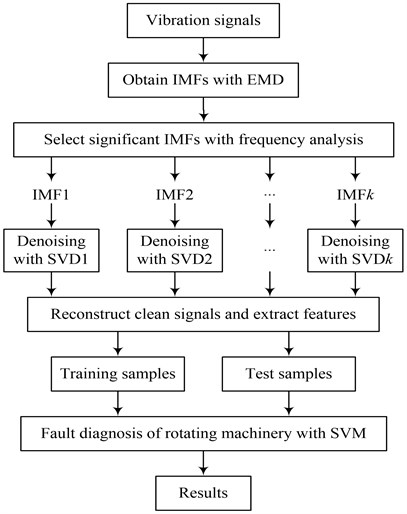
The proposed method mainly includes three steps: noise reduction, feature extraction and SVM based fault diagnosis, and its implementation process is shown in Fig. 1 and explained as following.

Fig. 1Implementation process of the proposed method

5. Experiment study

5.1. Experimental set up

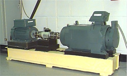
An experiment is carried out to validate the effectiveness of the proposed method using these data sets collected by the bearing data centre of the Case Western Reserve University [26]. The test bench includes a 2 hp motor, a torque transducer/encoder and control electronics which was not shown in Fig. 2. The motor shaft is supported by deep grove ball bearings (6205-2RS JEM SKF). The specifications (inches) of the used bearing are 0.9843, 2.0472, 0.3126 and 1.537 in inside diameter, outside diameter, ball diameter and pitch diameter, respectively. These test bearings include various single point faults introduced by electro-discharge machining. The considering bearing conditions are normal, inner ring fault, ball fault and outer ring fault. Vibration data sets of these considering conditions were collected by a 16 channel DAT recorder with accelerometers. By the formulas in paper [1], the CDFs of inner ring fault, ball fault and outer ring fault are 162.19 Hz, 107.36 Hz and 141.17 Hz, respectively. In this experiment, the speed of shaft is 1797 rpm, and just these data sets, obtained from these test bearings with various faults in 0.07 inches at a sampling frequency of 12000 Hz, are selected to testify the effectiveness of the proposed method.

Fig. 2Test bench

5.2. Results and discussion

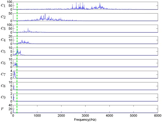
Fig. 3 shows the IMFs and residual of the vibration signal collected from the bearing under inner ring fault during 1/6 s sampling time. As shown in this figure, each decomposition component includes some local characteristics which can represent the information belonging to the corresponding bearing condition. However, without enough experience and professional skill, these bearing faults still cannot be accurately diagnosed by these decomposed IMFs. Therefore, if we can extract some useful features from these decomposition components, the fault diagnosis will be not so complicated. Further analysis of Fig. 3 shows that the main frequency of the front IMF is higher than that of the later one. The FFT waves of these IMFs plotted in Fig. 3 are showed in Fig. 4, where the dotted line means the minimum frequency of the calculated CDFs. From the plots in Fig. 4, it is obvious that the main frequency compositions of these IMFs in Fig. 3 distribute from high to low. Meanwhile, the major frequency components in the first 5 IMFs are higher than the frequency value showed by dotted line. At the same time, for other faulty conditions, we find that the first 5 IMFs also include the CDFs and other higher frequency components, and which are not plotted in this paper considering typography. Therefore, we select the first 5 IMFs for fault diagnosis and other ones are abandoned as noise.

Fig. 3IMF waves of a bearing under inner ring fault

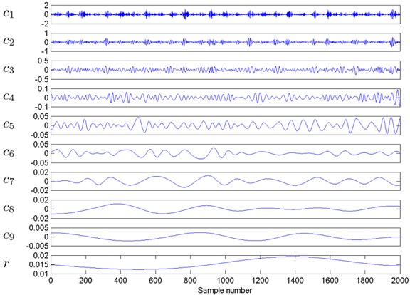
Fig. 4FFT waves of these IMFs plotted in Fig. 3

After these so-called noise components are canceled by removing some low-frequency IMFs and residue signal, SVD is used to do secondary noise reduction of these ‘clean’ IMF components. In [18], two rules were summarized from an experiment to determine the Hankel matrix size, and they are: if a signal has even $N$ data points, the Hankel matrix size should be $\left(N/2+1\right)\times N/2$; if a signal has odd $N$ data points, the Hankel matrix size should be $\left(N+1/2\right)\times \left(N+1/2\right)$. In this work, each of these selected vibration signal sections includes 2000 sampling points, so the column and row of the constructed Hankel matrix are 1000 and 1001, respectively. Fig. 5 illustrates the normalized singular values and their difference spectrum of IMF1 in Fig. 3, and it is obvious that the front singular values are bigger than the back ones. As the difference spectrum showing, most of the local peaks within the coordinates 1 to 200 are bigger than those between 201 and 1000, and the maximum peak is plotted in the 8th coordinate by considering the DC component effect of the first singular value [18]. If using the method described in [18] to cancel the noise of IMF1 in Fig. 3, the front 8 singular values are selected to reconstruct the clean signal. For the approach in [14], it is difficult to directly compute the derivation values of normalized singular plots. In fact, the maximum peak of these difference values of the difference spectrum of singular values can be regarded as the threshold point defined in [14]. Coincidentally, the reconstruct singular order is also 8 for the inner ring fault. However, these singular values with coordinate 9 to 100 are still very big, and this means that their reconstructed components may still include a great of useful information. To balance signal denoising and useful information highlighting, the so-called clean signal is constructed by these singular values whose number is equal to the biggest $X$ coordinate of this local difference spectrum peak which is no less than 0.1 time of the maximum peak determined by this method in [18]. Fig. 6 plots the reconstructed results of IMF1 in Fig. 3 using various methods: (a) method in [14] and [18]; (b) the proposed method. By the above discussion, the reconstructed signals of the methods in [14] and [18] are all overlap because their reconstructed singular values are the same. These plots in Fig. 6 shows that some impulse compositions have been removed as noise when the first 8 singular values are used to reconstruct the vibration signal of inner ring fault. However, the proposed method can reserve more useful details when doing signal noise reduction.

Fig. 5Normalized singular values and their difference spectrum of IMF1 in Fig. 3

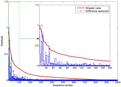
Fig. 6Reconstructed results of IMF1 in Fig. 3 using various methods: a) methods in [14] and [18]; b) the proposed method

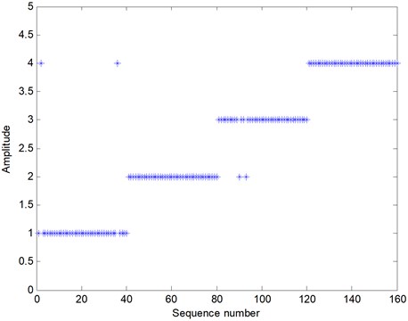
To diagnose bearing faults intelligently, SVM is carried out. For each bearing condition under load 1 to 4, we extract 60 samples: 20 ones for training the SVM model and other 40 ones for test. The detail parameters and code of the used SVM can be found in [27]. The labeled outputs of the SVM are: normal bearing (1), inner ring fault (2), ball fault (3) and outer ring fault (4). The experimental results of these test samples under load 1 is presented in Fig. 7. In this figure, test samples with number 1-40, 41-80, 81-120 and 121-160 are under these bearing conditions of normal, inner ring fault, ball fault and outer ring fault, respectively. As shown in this figure, two outputs of test samples with number 1-40 are 4 and others are all 1, and this means that two test samples have been diagnosed wrongly. For these test samples with number 81-120, two outputs are 2 which should be 3, and this means that two test samples of ball fault are identified incorrectly. In addition, the other test samples are all exactly diagnosed. Therefore, the fault diagnosis accuracy (FDA) of bearings under load 1 is 97.50 %. By the same way, the FDAs of bearings under load 2 to 4 are 98.75 %, 98.75 % and 96.25 %, respectively. According to the above analysis, it can be seen that the proposed method can effectively diagnose bearing faults in a rotating machinery system.

Fig. 7Test results of SVM when bearings under load 1

6. Conclusions

In this paper, a new method using empirical mode decomposition (EMD) and singular value decomposition (SVD) to obtain clean signals were proposed to diagnose the faults of rotating machinery, and which also involves a support vector machine (SVM) model. EMD was applied to decompose the obtained vibration signals into several intrinsic mode functions (IMF) at first. To cancel the noise hidden in the vibration signals, only these IMFs including the CDFs and higher frequency components were then selected to do further noise reduction using SVD, and other IMFs were abandoned as noise. Then the so-called clean IMFs were added together as the clean signal for features. Finally, the test features were used to verify the SVM model constructed by training samples. The experimental results testified that the proposed method was effective in mechanical fault diagnosis.