Non-stationary vibration studying based on singular spectrum analysis

1. Introduction

Singular spectrum analysis (SSA) is new powerful method of time series analysis and forecasting, which was independently developed in Russia (called “Caterpillar”- SSA) and also in UK and USA (under the name of SSA) [1-4]. The “Caterpillar” – SSA is a model-free technique of time series analysis; it combines advantages of other methods, such as Fourier and regression analyses, with simplicity of visual control aids.

The “Caterpillar” – SSA approach is used to study the time series in many various spheres wherever the trend or periodic behaviour may present: in meteorology, climatology, hydrology, geophysics, medicine, biologyy, sociology. A lot of problems can be solved by means of “Caterpillar” – SSA technique: finding trends of different resolution, smoothing, extraction of the periodic components, change-point detection, simultaneous extraction of cycles with small and large period; extraction of periodicities with varying amplitudes. Method is extensively developing: the modification of SSA for time series with missing data and the variants for analysis of multidimensional time series (MSSA) are elaborated.

Last decade the methods for nonstationary and nonlinear time series based on Empirical Mode Decomposition (EMD) are developed. EMD method used to decompose series as sums of zero-mean components. The technique consists basically of computing an upper and lower spline envelope of the time-series and extracting the average of this envelope up to when the residuals are random noise or stopping criterion is met. SSA method is more mathematically grounded, while EMD is more empirical. The aim of SSA is to make a decomposition of the original series into the sum of independent and interpretable components: trend – sum of slowly varying components, oscillatory components – sum of elementary harmonic components and a structureless noise – the random component formed by a set of random factors.

The “Caterpillar” – SSA method is useful tool for short and long, stationary and nonstationary, almost deterministic and noisy time series analyzing. The method can be successfully used for processing the signals from the vibrating constructional elements and machine parts. However, in mechanics application this method does not become widely used, but it may be successfully used for periodic motion detection, amplitude and frequency definition, as well as chaotic motion identification. The purpose of this work is to show the principle of the method, its ease of use and accessibility for mechanical applications. For this purpose the examples of vibration of construction element is considered: nonstationary vibration of pier abutment under seismic action.

2. Mathematical background

The main steps of “Caterpillar” – SSA algorithm described here, follow the methodology given in work [3]. The basic version of method consists in transformation of one-dimensional series into multi-dimensional by one-parametric translation procedure, research of got multidimensional trajectory by means of principal components analysis (Singular Value Decomposition) and reconstruction of the series in accordance with the chosen principal components. The result of this method application is expansion of the time series into sum of simple components: slow trends, periodic or oscillating components and components of noises. The obtained decomposition may serve as basis of correct forecasting. Both of two complementary stages of SSA technique (decomposition and reconstruction) include two separate steps, therefore the analysis is performed by four steps.

At the first step (called the embedding step) a one-dimensional series $F=(f_0,...,f_{N-1})$, $f_n\in \mathbb{R}$, with length $N\ge 3$ is transferred to the $L$ – dimensional vector:

where $K=N-L+1$ and $1<L<N\text{,}$$L\in \mathbb{N}$. $L$ is called by window length, it is very important parameter of the embedding step; it should be big enough but not greater than a half of series length. This delay procedure gives the first name to the whole technique.

Vectors ${\mathbf{X}}_i$ form columns of the trajectory matrix $\mathbf{X}=\left[X_1:\dots :X_K\right]$, or:

Trajectory matrix $\mathbf{X}$ is a Hankel matrix, which mean that all the elements along the diagonal $i+j=const$ are equal: $x_{ij}=f_{i+j-2}$.

The second step is the singular value decomposition (SVD) of the trajectory matrix into a sum of rank-one bi-orthogonal elementary matrices: $\mathbf{X}={\mathbf{X}}_1+\dots +{\mathbf{X}}_d.$

Elementary matrix ${\mathbf{X}}_i$ is determined by the equality:

where $\sqrt{{\lambda }_i}$ ($i$-th singular value) is the square root of the $i$-th eigenvalue of the matrix $\mathbf{S}$, ${\mathbf{U}}_1\text{,...,}{\mathbf{U}}_L$ – orthonormal set of eigenvectors of matrix $\mathbf{S}$, $d=\mathrm{m}\mathrm{a}\mathrm{x}\{i:\lambda i>0\}$, ${\mathbf{V}}_i={\mathbf{X}}^T{\mathbf{U}}_i/\sqrt{{\lambda }_i}$. ${\mathbf{U}}_i$ and ${\mathbf{V}}_i$ are called as left and right singular vectors of the trajectory matrix. It is assumed that eigenvalues ${\lambda }_i$ are arranged in decreasing order of their magnitude$\left({\lambda }_1\ge \dots \ge {\lambda }_L\ge 0\right)\text{.}$ The collection $\left(\sqrt{{\lambda }_i,}{\mathbf{U}}_i,{\mathbf{V}}_i^T\right)$ is called the $i$-th eigentriple of matrix $\mathbf{X}$.

The third step (grouping step) corresponds to splitting of the elementary matrices ${\mathbf{X}}_i$ into several groups and sunning the matrices within each group. Grouping procedure splits the set of indexes $\{1,\dots ,d\}$ into the disjoint subsets $I_1\text{,}{I}_2\text{,...,}{I}_m\text{.}$ Let $I_k=\{i_1,...,i_p\}$ then ${\mathbf{X}}_{I_k}={\mathbf{X}}_{i_1}+...+{\mathbf{X}}_{i_p}$ under condition $I={\bigcup }_{k=1}^m{I}_k$. For given group $I_k$ the contribution of the component ${{\mathbf{X}}_I}_k$ into the expansion is measured by the share of the corresponding eigenvalues.

The last step (diagonal averaging) transfers each resultant matrix into a Hankel matrix, from which then the time series will be reconstructed (the additive components of the initial series $F$). Let $y_{ij}$ stands for an element of $L\times K$ matrix $\mathbf{Y}\text{,}$ where $1\le i\le L\text{,}$$1\le j\le K\text{.}$ Let $L^{*}=\mathrm{m}\mathrm{i}\mathrm{n}\left(L,K\right)\text{,}$$K^{*}=\mathrm{m}\mathrm{a}\mathrm{x}\left(L,K\right)\text{,}$$y_{ij}^{\mathrm{*}}=y_{ij}$ if $L<K$ and $y_{ij}^{\mathrm{*}}=y_{ji}$ otherwise. Diagonal averaging transforms matrix $\mathbf{Y}$ into series $g_0\text{,...,}{g}_{N-1}$ ($N=L+K-1$) by formulas:

Elements of Hankel matrix is obtained by averaging of $y_{ij}$ over all $i\text{,}$$j$ such that $i+j=k+2$. In this way we obtain a decomposition of the initial series into several additive components. The result is the expansion of matrix ${\mathbf{X}}_{I_k}$ into simple components $F^{\left(k\right)}=\left(f_0^{\left(k\right)},\dots ,f_{N-1}^{\left(k\right)}\right)$ and initial series $F=\left(f_0,\dots ,f_{N-1}\right)$ is decomposed into the sum of $m$ series:

Forecasting time series, unlike the analysis, is only possible involving the mathematical model of the series. The model must either originate from the data itself, or be tested on the available data. When forecasting with SSA method, we consider a set of time series described by linear recurrent formula (LRF). The class of time series governed by linear recurrent formulae is rather wide; it includes harmonics, polynomial and exponential time series. The time series governed by LRF generates recurrent extension as each its term is a linear combination of some of the previous ones. SSA forecasting method can be applied to the time series that approximately satisfy linear recurrent formulas.

For SSA procedure the correct choosing of window length $L$ and way of grouping of of the eigentriples (or grouping of elementary matrices, since each matrix component of the SVD is completely determined by the corresponding eigentriple) are very important. It is preferable to take the window length proportional to supposed period in order to achieve the better separability of the periodic components. As for the way of grouping, it is useful to mention that under the proper choice of window length $L$ singular vectors ‘repeat’ the behavior of corresponding time series components. In particular, trend of the series corresponds to slowly varying singular vectors; harmonic component produces a pair of left (and right) harmonic singular vectors with the same frequency, etc.

The main principles for identification of eigentriples corresponding to the time series component of interest are as follows: to extract the trend or to smooth the time series, slowly changing eigenfunctions are chosen; to extract oscillations, oscillating eigenfunctions are chosen; to extract harmonic components with period greater than 2 a pair of eigentriples with the same period should be found and chosen; to approximate the time series the leading eigentriples are chosen.

3. Numerical examples of SSA method application

In recent years corresponding computer software are elaborated for time series analysis: “Caterpillar” – SSA and Rssa package in St. Petersburg University [1, 3], SSA-MTM Toolkit for Spectral Analysis, kSpectra Toolkit [5]. MATLAB program is also widely used. In this work MathCAD program are applied as easy-to-use environment for engineers and scientists research. MathCAD has a large number of built-in functions, including matrix, and programming tools. The analysis of horizontal and vertical displacement of the top of pier after seismic action is performed by means of “Caterpillar” – SSA method using MathCAD. Recording of the amplitudes (mm) was made with regular interval 0.04 s, hereinafter this data are called as time series.

3.1. Example 1

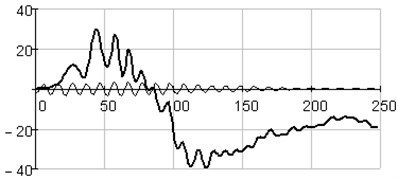
The analysis of horizontal vibration of the pier top is presented below, time series length is equal 248 ($N=$ 248). Initial time series and its trend (reconstructed with the first 4 eigentriples) are presented in Fig. 1, window length is set $L=$ 124. Plot in Fig. 2 shows the plot logarithms of eigenvalues in decreasing order; logarithm was introduced because of very large figures.

It is clear that the first four eigenvalues have the largest value and are able to explain the main part of variance. To determine the size of informative basis the next features of eigenvalue is used: the larger share of eqenvalue in the sum of elements of the eigenvalues vector, the more background information includes a projection on the corresponding eigenvector. Because a drop in values is observed around 14-th eigenvalue, it may be supposed that there noise floor starts.

Plot in Fig. 2 may be used for periodical components finding. Since in ideal situation two main components with the same period (“sin” and “cos”), relevant to one eigenvalue, correspond to one sinusoidal component, in real situation these components correspond to close eigenvalues. Thus the “tread” may be observed in the plot: 5-6, 7-8, 9-10, 11-12, i.e. four evident pairs, with almost equal leading singular values.

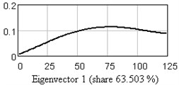
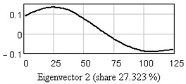
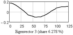
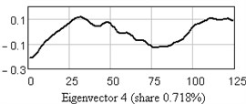
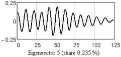
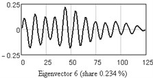
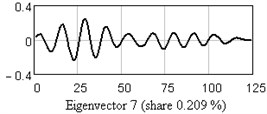
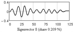
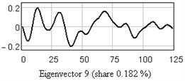
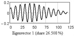
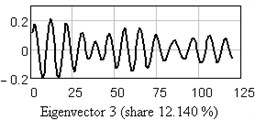
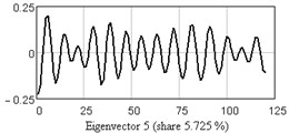
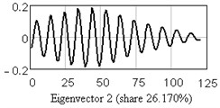
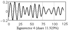
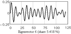
In Fig. 3 one-dimensional plots of the first nine eigenvectors are given as the example. Analysis of eigenvectors shows that the first four eigenvectors are a trend components (slowly changing component), the 5-6 and 7-8 may be periodical components.

Fig. 1Initial series () and its trend (), reconstructed with first four eigentriples

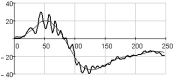
Fig. 2Singular value spectrum: plot of logarithms of the first 60 from 124 eigenvalues

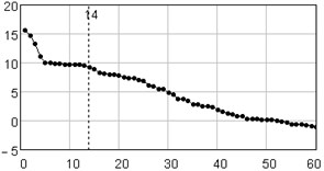
Fig. 3One-dimensional plots of the first nine eigenvectors

a)

b)

c)

d)

e)

f)

g)

h)

i)

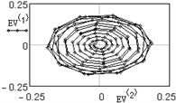
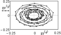
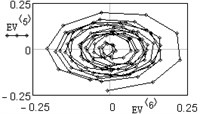
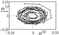
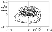
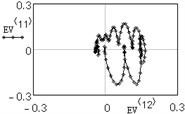
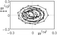
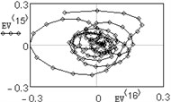
Fig. 4 shows the examples of two-dimensional projection of the eigenvectors; vectors number is indicated in superscript of function and argument. Analysis of plots in Fig. 4 confirms the conclusion that the 5-th and 6-th eigenvectors (and also 7-th and 8-th) refer to the periodical components.

In Fig. 5(a) the periodical components consisting of the 5-th and 6-th eigentriples is presented, in Fig. 5(b) – sum of periodical components from 5-th to 12-th eigentriples.

By the same way the rest eigenvectors may be investigated.

Fig. 4Two-dimensional plots of eigenvectors

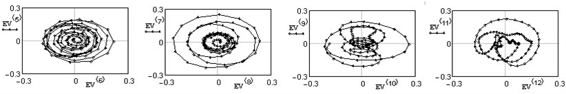
Fig. 5Plots of the initial series () and periodical components (): a) reconstructed with 5-th and 6-th eigentriples, b) reconstructed with eigentriples from 5-th to 12-th

a)

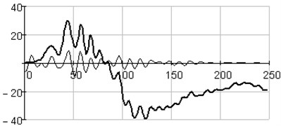
b)

3.2. Example 2

The analysis of vertical vibration of the pier top is presented in Figs. 6-11; time series length $N=$242, window length is set $L=$ 120. Initial time series is presented in Fig. 6, plot in Fig. 7 shows the logarithms of eigenvalues in decreasing order; after 14-th component the drop in value occurs, it could be considered as start of the noise floor. Six evident pair with almost equal leading singular value correspond to six (almost) harmonic components of series: eigentriples pair 1-2, 3-4, 5-6, 7-8, 9-10 and 13-14 are related to the harmonic components. Reconstructed series with first 14 eigentriples is given in Fig. 8, reconstructed series of noise (last 106 eigentriples) – in Fig. 9. The principal components of first six eigentriples are shown in Fig. 10, two-dimensional plots of eigenvectors is given in Fig. 11.

This scatterplots of paired principal components tend to a center, it means that vibrations are damped. For non-damped vibration two-dimensional plot appears as ring or circle. From this plots it is seen that eigenvectors 11-12 are not periodical components.

Fig. 6Initial series of amplitudes

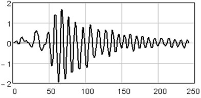
Fig. 7Singular value spectrum: plot of logarithms of the first 40 from 120 eigenvalues

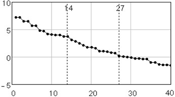
Fig. 8Reconstructed series with first 14 eigentriples (periodical components)

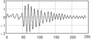
Fig. 9Noise reconstructed series (15-120 eigentriples)

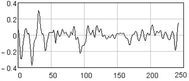
Fig. 10One-dimensional plots of the first six eigenvectors

a)

b)

c)

d)

e)

f)

Fig. 11Two-dimensional plots of eigenvectors

a)

b)

c)

d)

e)

f)

g)

h)

4. Conclusions

Examples of application of the SSA technique for analysis of one-dimensional time series is presented in this work: task of analysis of nonlinear vibration of the elements of constructions under seismic action. Simple solution shows the convenience of this method, its usability to nonstationary time-series investigation.

References

-
Danilov D., Zhigljavsky A. Principal Components of Time Series: “Caterpillar” Method. St. Petersburg University, St. Petersburg, Russia, http://www.gistatgroup.com/gus/, 1997.
Ghil M., et al. Advanced spectral methods for climatic time series. Reviews of Geophysics, Vol. 40, 2002, p. 1-1–1-41.
Golyandina N., Zhigljavsky A. Singular Spectrum Analysis for Time Series. Springer Briefs in Statistics, Springer, 2013.
Jolliffe I. T. Principal Component Analysis. Springer-Verlag, 1986.
SSA –MTM Toolkit for Spectral Analysis, http://www.atmos.ucla.edu/tcd/ssa/.
About this article