Abstract
This paper deals with the problem of gear fault diagnosis with multiple possible fault modes and damage levels. Gears are the most essential parts in rotating machinery. Their health status is a significant index to indicate whether machines can run continually or not. So, gear fault diagnosis and damage level identification is very important in engineering practice. An accuracy way to identify the state of gears is urgently needed for the maintenance decision making. In this paper, a novel gear fault diagnosis and damage level identification method based on Hilbert transform (HT) and Euclidean distance technique (EDT) is developed. The energies of six frequency bands are used as the fault feature through the contrast with other two parameters, kurtosis and skewness. Then HT is used to obtain analytic signal. Finally, EDT is utilized to recognize the different fault modes and damage levels. This method is implemented by two stages, i.e., classifying different fault modes and identifying damage levels for every fault mode. The effectiveness of this methodology is demonstrated by compare to fisher discriminant analysis (FDA) using experiment data acquired from a real gearbox. In addition, industrial data is also used to validate the effectiveness of the proposed method.
1. Introduction
Gearboxes are widely used in rotating machinery for mechanical transmission, and failures of gears usually cause significant loss in terms of unavailability and maintenance of the machines. Therefore, there is a constant need to reduce gear breakdown and maintenance costs. So far, the most efficient way of reducing the costs would be to monitor the condition of these systems. Early fault diagnosis and damage level identification are key problems to be solved, and become increasingly important in condition monitoring. To this end, many techniques have been used in fault diagnosis. Such as Empirical Mode Decomposition (EMD) [1, 2], Support Vector Machine (SVM) [3, 4], Hilbert-Huang Transform (HHT) [5], Wavelet Packet Transformation (WPT) [6] and Hidden Markov Model (HMM) [7-9]. As the equipments becoming more and more complicated, sometimes the problem cannot be solved by using only one technique. Hereby, the combination of two or three of them may be utilized.
Samuel and Pines [10] reviewed the research state in vibration-based techniques for helicopter transmission diagnostics. They illustrated the importance of condition monitoring for gearbox from the view of cost and safety. Saravanan and Ramachandran [11] used a discrete wavelet features and decision tree classification method to detect the faults of spur bevel gearbox. Fan and Zuo [12] proposed a fault detection method that combines Hilbert transform and wavelet packet transform to extract modulating signal and help to detect the early gear fault. In recent years, many researchers pay more attention to the fault feature extraction methods. Documents [13] and [14] introduced the normal used feature parameters including energy, kurtosis and skewness etc. Casimir etc. [15] developed a model based on features selection and nearest neighbors rule to deal with the diagnosis of induction motors. An intelligent diagnosis for fault gear identification and classification based on vibration signal using discrete wavelet transform and adaptive neuro-fuzzy inference system (ANFIS) was proposed in [16] for solving the problem of abnormal transient signals. This enabled the fault characteristic frequency of gears can be detected effectively. Lei and Zuo [17] proposed a new algorithm in classifying the different levels of gear cracks based on weighted K nearest neighbor. A comparative study on classification of features by SVM and PSVM extracted using Morlet wavelet was developed in [18] for fault diagnosis of spur bevel gearbox. Kim and Zuo [19] considered the problem of fault diagnosis for a system with many possible fault types and proposed two fault classification methods for large systems when available data are limited. And the two methods are fault tree and bayes classification approach. In recent years, many pattern recognized methods are used in fault diagnosis field, such as Fisher discriminant analysis [20, 21].
These methods mentioned above are very effective to determine the fault of gears. However, some of them were mainly deal with the problem of fault mode classification and others were aimed at damage level identification. None of them solve the two issues together. In engineering practice, these problems usually occur coincidently. In order to solve the dilemma, this paper developed a gear fault diagnosis and damage level identification method based on Hilbert transform (HT) and Euclidean distance technique (EDT). This method can distinguish the different fault modes and recognize different damage levels for every fault mode at the same time. And the performance of the method has been tested.
The remaining sections of this paper are organized as follows. In Section 2, the framework of the proposed method was given out and the theory of EDT and HT were introduced. Section 3 described the experiment, the procedure of training model and results analysis. Section 4 validated the proposed method using industrial data. Finally, the conclusions were drawn in Section 5.
2. Methodology
2.1. Framework of the proposed method
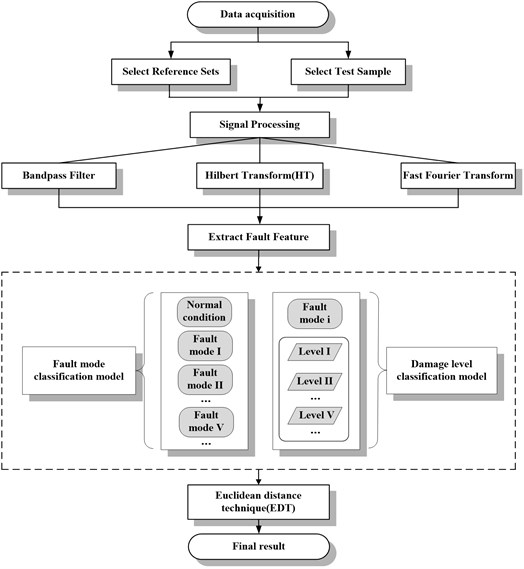
The method this study proposed is mainly made up of two stages: classify different fault modes and identify damage levels of every mode. Fig. 1 shows the framework of the method this paper proposed.
In the method, data acquisition should be completed at the beginning of the study. In this research, experimental data of gearbox are mainly utilized. Four accelerometers are used to collect vibration signal. Meanwhile, reference sets and test samples should be selected. Historical data can be chosen as the reference sets when use the method this paper proposed. But in this study, the reference sets and test samples are all acquired from the experimental data. Several processes should be done after determining the data this study used. This paper mainly used band pass filter, Hilbert transform (HT) and Fast Fourier transform (FFT), the function of them is decrease disturb and make contribute to fault feature extraction. Fault features are the key factors affecting the model performance. Since if the appropriate parameter is selected, then the method will be effective in a great extent. Three fault features have been contrasted in this study. Finally, the energies of frequency bands are selected as the fault feature. The energies of frequency bands are used as the fault feature in this approach. Since this is a two stages method, two classification models are needed.
The purpose of the first classified model is to distinguish the health states of the gearbox, including normal condition, gear breaktooth and crack. This is foundation of this two-stage method.
For every sample, if a fault mode is identified, then the second classification model is employed. The function of it is to discriminate different damage levels of every mode. In the following study, the levels of breaktooth and crack are 2 mm, 5 mm, 10 mm and 2 mm, 5 mm, 8 mm, respectively.
EDT is used in the two models, the minimum distance between test sample and reference sets denote the type of the test sample. For example, if the distance between a test sample and normal condition is shorter than the others, then the test sample is normal.
After a test sample calculated by the two model, the optimum state (i.e. fault mode and damage level) of it will be determined. Maintenance decisioncan could be made based on this result. This is the theory of the method.
Fig. 1Framework of the method this paper proposed
2.2. Euclidean distance technique
Euclidean distance technique (EDT) is one of the pattern recognition methods widely used in image processing. The most fundamental investigative issue of pattern recognition is the similarity problem between samples as well as classes. Judging the similarity between samples often use nearest standard, i.e. compare test samples with reference sets and the sample belong to the class which has the high similarity with it. The usually used pattern recognition methods are euclidean distance, mahalanobis distance, cosine distance etc. Euclidean distance technique (EDT) was mainly used in this paper.
Assume there are two samples , . They can be denoted as:
Fig. 2(a) shows that these two samples are belong to same class because the distance between them is very short. On the contrary, these two samples are belong to different classes due to its long distance as depicted in Fig. 2(b).
And the Euclidean distance can be defined as:
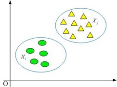
Fig. 3 shows the Euclidean distance between and Class . There are two ways to calculate the Euclidean distances between the test sample and class, as follows:
(1) Calculate the Euclidean distances between the test sample and every sample in Class , and then get the mean value of these distances as the euclidean distance between and Class :
where is the total number of the samples which in Class .
(2) First, get the center point of the samples in Class , and then calculate the euclidean distance between the test sample and as the Euclidean distance between and Class :
This paper chooses the first method as the calculate equation of the euclidean distance between and Class .
Fig. 2The class that the samples belong to: a) same class, b) different class
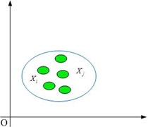
a)
b)
It is assumed that there are classes: , ,…, . Each class contains samples. For example, the class can express as . If we want to know which class the sample belongs to, the distances between this sample and every classes need to be calculated.
If the results satisfy the condition:
Then, it can be infered which class this vector belongs to.
Fig. 3Euclidean distance between sample and class
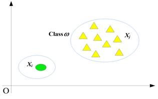
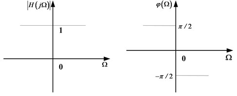
Fig. 4The amplitude and phase frequency characters of HT
2.3. Hilbert transform
In order to obtain analytic signal and make Euclidean distance computation more accquracy, Hilbert transform should be implemented. Assume the original signal is , the Hilbert transform of it can defined as:
can be seen as the output of pass through a filter, and the unit impulse respond of this filter is . Then, according to the Fourier transform (FT) theory, the FT of is , so:
If , then and:
That is to say, after Hilbert transform (HT), the discrete negative frequencies of signal overturn with +90° and the positive frequencies overturn with –90°. The amplitude and phase frequency characters of HT as shown in the Fig. 4.
is the HT of , define as follows:
Then, is the analytic signal of .
3. Experiment and data analysis
3.1. Experiment specifications
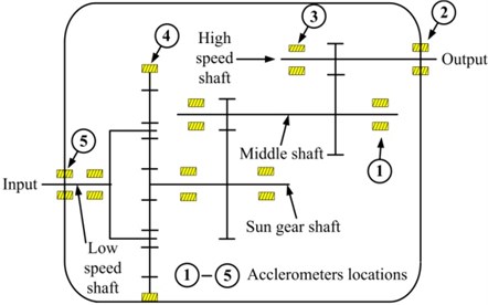
Fig. 5The structure of gearbox this experiment used and acclerometers locations
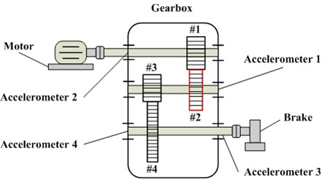
The data utilized in this study is obtained from the RCM laboratory of Mechanical Engineering College. The sampling frequency of this experimental system is 20 kHz and sampling time is 6 s. Each fault mode has 60 samples. The input rotary speed of motor is 800 rpm and the load generated by brake is 10 N∙m. Fig. 5 shows the structure of the gearbox used in this experiment and the acclerometers locations. The #2 gear is test gear, the tooth number of which is 64. The numbers of other three gears are 35 (#1), 18 (#3) and 81 (#4). The specific samples this study used will be introduced in next section.
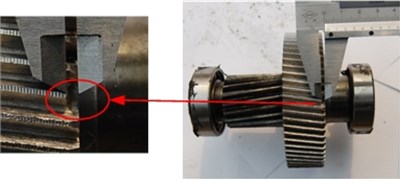
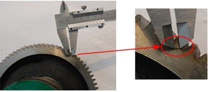
The maching method is used to introduce faults to the test gears. And the faults were planted using different fault modes (gear breaktooth and crack). Each mode has different levels, and the diameters of faults are 2 mm, 5 mm, 10 mm and 2 mm, 5 mm, 8 mm, respectively. The fault gears uesd in this study was shown in Fig. 6. In particular, (a) and (b) are the represents of breaktooth and crack, the damage length of them is 2 mm.
Fig. 6The fault gears used in this study
3.2. Model training
The training activities were performed using MATLAB signal processing in this study. And experimental data introduced above is mainly used.
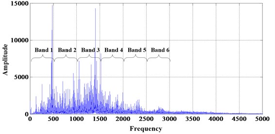
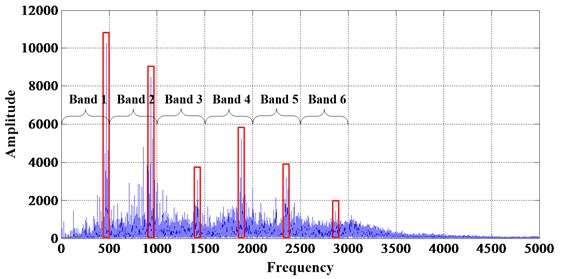
An obvious phenomena of fault gears is exist fault characteristic frequency and its multi-frequencies in amplitude spectrum. Figs. 7 and 8 shows the frequency spectrum of original signal, where Figs. 7 and 8 stand for the normal and breaktooth signal, respectively. And the phenomena can be seen directly by the comparison between them. So choose the energy of frequency band as feature and used to recognize the gear conditions is feasibility. Six filters are defined to obtain the energies of the six frequency bands based on the fault characteristic frequency and its multi-frequencies for the purpose of determining the characteristic vector. The six frequency bands are: band 1 [0-500 Hz], band 2 [500-1000 Hz], band 3 [1000-1500 Hz], band 4 [1500-2000 Hz], band 5 [2000-2500 Hz] and band 6 [2500-3000 Hz] (as Figs. 7 and 8 shows).
Fig. 7The frequency spectrum of original normal signal
After determining the six frequency bands, HT should be implemented. The function of this process has described in Section 2.3. Hereafter will not introduced any more.
The signal is a discrete series of numbers after processed by Hilbert transform technique. Discrete Fourier Transform (DFT) is needed to computing the signal frequency spectrum. For the purpose of reducing the amount of computations involved in the DFT, the Fast Fourier Transform (FFT) is used in this study.
Then the energy of every frequency band can be calculated. And the characteristic vector is constituted by the six numbers. Then, the reference sets and test samples should be selected. Every fault type has 60 samples as described above, the 1-10 samples of every fault mode and level is selected as the reference sets and the 11-40 samples are choosen as the test samples in this approach. The results of three reference sets which belong to normal condition, breaktooth and crack constitute the characteristic matrix of fault modes. Then the euclidean distances between test sample and each vector in the characteristic matrix can be computed. At first, ten euclidean distances between test sample and each mode reference sets are calculated. Then compute the mean value of the ten numbers. Finally, compare the three mean value and the fault modes can be identified. Similarly, the damage levels are classified utilizing the same procedure.
Fig. 8The frequency spectrum of original breaktooth signal
3.3. Results analysis
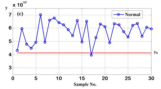
Following the training procedure in Section 3.2, fault diagnosis and damage level can be identified using the trained model. Firstly, normal condition and two kinds of fault modes (gear breaktooth and gear crack) are distinguished. Due to the importance of selecting fault feature, this paper choosed three parameters (kurtosis, skewness and energy) to detect which is more effective. Figs. 9, 10 and 11 are the results of the three features, the distances are all mean value described above, similarly hereafter.
Fig. 9Distances between test samples and reference sets extract kurtosis as feature value
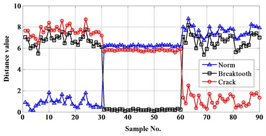
The importance of selecting fault feature can be seen from Figs. 9-11. If skewness is choosen as the feature, then it is impossible to distinguish the fault modes with a high successful rate. Either kurtosis or energy is okay, but the result of energy is more ideal than kurtosis. So, energy is selected as the feature in this approach.
In order to test and verify the necessity of dividing frequency bands, the distances of the whole energy were also calculated. Fig. 12 shows the result when the bandpass filters were not designed. The result indicate that the accuracy rate is much lower than before. So it is important to define frequency bands when Euclidean distance technique (EDT) is utilized.
Fig. 10Distances between test samples and reference sets extract skewness as feature value
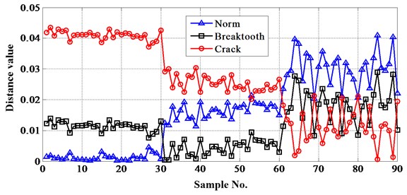
Fig. 11Distances between test samples and reference sets extract energy as feature value
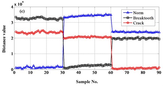
Fig. 12The result when the frequency bands were not designed
The specific distance values when select energy of frequency band as fault feature can be seen in Table 1.
For the purpose of verify the method this paper proposed, Fisher discriminant analysis (FDA) is used to do the same work. Fisher discriminant analysis is mainly used to solve the “Dimension disaster” problem which often confront in pattern recognition field, some methods are applicative when in high dimension space but they do not work in below dimension space. However, many methods are more accurate in high dimension space than below. This moment dimension reduction can achieve very good results and it is the objective that utlize FDA.
Table 1Distances between test samples and reference sets
Case no. | Norm | Breaktooth | Crack | Case no. | Norm | Breaktooth | Crack |
1 | 1.02E+03 | 3.35E+04 | 2.41E+04 | 46 | 3.47E+04 | 2.87E+03 | 2.09E+04 |
2 | 9.09E+02 | 3.24E+04 | 2.35E+04 | 47 | 3.43E+04 | 2.14E+03 | 2.02E+04 |
3 | 1.08E+03 | 3.25E+04 | 2.33E+04 | 48 | 3.48E+04 | 2.71E+03 | 2.13E+04 |
4 | 1.10E+03 | 3.22E+04 | 2.35E+04 | 49 | 3.42E+04 | 2.42E+03 | 2.09E+04 |
5 | 2.67E+02 | 3.29E+04 | 2.40E+04 | 50 | 3.47E+04 | 2.64E+03 | 2.11E+04 |
6 | 1.14E+03 | 3.19E+04 | 2.32E+04 | 51 | 3.46E+04 | 2.48E+03 | 2.08E+04 |
7 | 1.23E+03 | 3.24E+04 | 2.31E+04 | 52 | 3.48E+04 | 2.85E+03 | 2.07E+04 |
8 | 2.20E+03 | 3.23E+04 | 2.25E+04 | 53 | 3.47E+04 | 2.63E+03 | 2.05E+04 |
9 | 1.54E+03 | 3.18E+04 | 2.32E+04 | 54 | 3.47E+04 | 2.95E+03 | 2.06E+04 |
10 | 1.41E+03 | 3.25E+04 | 2.31E+04 | 55 | 3.43E+04 | 2.28E+03 | 2.02E+04 |
11 | 7.54E+02 | 3.24E+04 | 2.36E+04 | 56 | 3.45E+04 | 2.58E+03 | 2.08E+04 |
12 | 2.40E+03 | 3.29E+04 | 2.28E+04 | 57 | 3.53E+04 | 3.29E+03 | 2.10E+04 |
13 | 7.85E+02 | 3.26E+04 | 2.36E+04 | 58 | 3.47E+04 | 2.89E+03 | 2.04E+04 |
14 | 9.82E+02 | 3.35E+04 | 2.42E+04 | 59 | 3.50E+04 | 3.06E+03 | 2.06E+04 |
15 | 1.02E+03 | 3.34E+04 | 2.47E+04 | 60 | 3.49E+04 | 2.73E+03 | 2.07E+04 |
16 | 1.36E+03 | 3.32E+04 | 2.36E+04 | 61 | 2.42E+04 | 1.98E+04 | 8.63E+02 |
17 | 9.47E+02 | 3.36E+04 | 2.46E+04 | 62 | 2.39E+04 | 1.99E+04 | 4.18E+02 |
18 | 1.62E+03 | 3.29E+04 | 2.49E+04 | 63 | 2.44E+04 | 1.95E+04 | 3.74E+02 |
19 | 1.04E+03 | 3.24E+04 | 2.40E+04 | 64 | 2.40E+04 | 1.97E+04 | 2.37E+02 |
20 | 1.30E+03 | 3.22E+04 | 2.33E+04 | 65 | 2.38E+04 | 2.00E+04 | 3.94E+02 |
21 | 1.47E+03 | 3.19E+04 | 2.31E+04 | 66 | 2.43E+04 | 1.93E+04 | 5.66E+02 |
22 | 1.17E+03 | 3.24E+04 | 2.39E+04 | 67 | 2.40E+04 | 1.91E+04 | 7.78E+02 |
23 | 1.52E+03 | 3.23E+04 | 2.41E+04 | 68 | 2.43E+04 | 1.99E+04 | 4.05E+02 |
24 | 1.32E+03 | 3.22E+04 | 2.37E+04 | 69 | 2.37E+04 | 2.02E+04 | 7.54E+02 |
25 | 1.09E+03 | 3.24E+04 | 2.40E+04 | 70 | 2.40E+04 | 1.94E+04 | 4.84E+02 |
26 | 1.72E+03 | 3.19E+04 | 2.31E+04 | 71 | 2.38E+04 | 2.00E+04 | 7.85E+02 |
27 | 2.26E+03 | 3.14E+04 | 2.33E+04 | 72 | 2.38E+04 | 1.98E+04 | 9.95E+02 |
28 | 1.45E+03 | 3.22E+04 | 2.35E+04 | 73 | 2.40E+04 | 2.00E+04 | 6.73E+02 |
29 | 1.46E+03 | 3.29E+04 | 2.45E+04 | 74 | 2.40E+04 | 1.95E+04 | 8.91E+02 |
30 | 1.61E+03 | 3.21E+04 | 2.38E+04 | 75 | 2.42E+04 | 1.97E+04 | 2.73E+02 |
31 | 3.34E+04 | 9.78E+02 | 1.99E+04 | 76 | 2.38E+04 | 2.02E+04 | 9.04E+02 |
32 | 3.32E+04 | 7.32E+02 | 1.99E+04 | 77 | 2.36E+04 | 2.05E+04 | 9.97E+02 |
33 | 3.31E+04 | 8.25E+02 | 2.01E+04 | 78 | 2.42E+04 | 1.91E+04 | 8.80E+02 |
34 | 3.36E+04 | 1.18E+03 | 2.04E+04 | 79 | 2.38E+04 | 1.98E+04 | 1.28E+03 |
35 | 3.38E+04 | 1.53E+03 | 2.04E+04 | 80 | 2.39E+04 | 2.03E+04 | 6.67E+02 |
36 | 3.41E+04 | 1.68E+03 | 2.06E+04 | 81 | 2.39E+04 | 2.00E+04 | 6.80E+02 |
37 | 3.36E+04 | 1.47E+03 | 2.03E+04 | 82 | 2.43E+04 | 1.93E+04 | 4.49E+02 |
38 | 3.39E+04 | 1.90E+03 | 2.09E+04 | 83 | 2.37E+04 | 1.99E+04 | 7.24E+02 |
39 | 3.39E+04 | 1.68E+03 | 2.06E+04 | 84 | 2.36E+04 | 2.02E+04 | 9.56E+02 |
40 | 3.42E+04 | 2.29E+03 | 2.12E+04 | 85 | 2.37E+04 | 2.01E+04 | 6.75E+02 |
41 | 3.42E+04 | 2.09E+03 | 2.08E+04 | 86 | 2.35E+04 | 1.95E+04 | 1.04E+03 |
42 | 3.43E+04 | 2.56E+03 | 2.09E+04 | 87 | 2.36E+04 | 2.01E+04 | 1.18E+03 |
43 | 3.45E+04 | 2.45E+03 | 2.08E+04 | 88 | 2.39E+04 | 1.98E+04 | 1.29E+03 |
44 | 3.43E+04 | 2.68E+03 | 2.10E+04 | 89 | 2.40E+04 | 2.00E+04 | 4.12E+02 |
45 | 3.43E+04 | 2.33E+03 | 2.04E+04 | 90 | 2.38E+04 | 1.94E+04 | 1.24E+03 |
The minimum numbers (in bold) represent the optimum state of test samples. It can be seen that the accurate rate of this method is 100 %. | |||||||
If there are many classes need to classified, two classes FDA should be implemented at first when identify a test sample, it will give out the nearest class which the test sample belong to. Then the nearest class and another new class could constitute a conference samples and conduct the two classes FDA, a new nearest class can be obtained, continue carry out the procedure above until all the classes are considered. At last, the class which the test sample belong to will be classified. As Fig. 13(a) shows, the red line is the threshold value (as same as the follows) which computed based on the specific data. The same to say, the value is not constant to the different analytical data. For example, is –7.47∙1016 and –3.90∙1016 in Fig. 13(a) and (b). First, select breaktooth and normal as class 1 and class 2, respectively. So if the projective value of one sample greater than , the sample belong to class 1, otherwise the sample belong to class 2. Namely, after the first comparison, the black and pink samples belong to class 1 (i.e. breaktooth) and the blue samples belong to class 2 (i.e. normal). Then the neareat class and crack constitute the reference sets. Similarly, (b), (c) are breaktooth-crack and normal-crack. The conclusion could be given out. Blue belong to normal, black belong to breaktooth and pink belong to crack. All the 90 samples, there are 10 samples are mistake. So the accurate rate of this method is approximate 89 %.
Fig. 13The result figures of gear fault modes diagnosis when use FDA
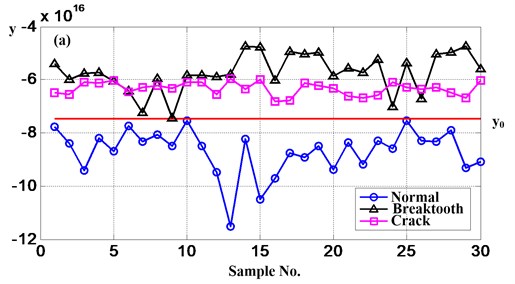
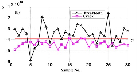
It is obviously that the accurate rate of FDA is lower than use the method this paper proposed, so the method based on Hilbert transform and Euclidean distance technique is effective.
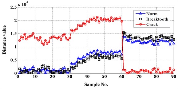
Along with the known of fault modes, the damage level of every mode can be recognized using the same technique. The results are shown in Fig. 14 and 15, where the detailed damage levels are identified, including breaktooth (2 mm, 5 mm and 10 mm) and crack (2 mm, 5 mm and 8 mm), respectively.
Fig. 14Distances between test samples and reference sets belong to breaktooth
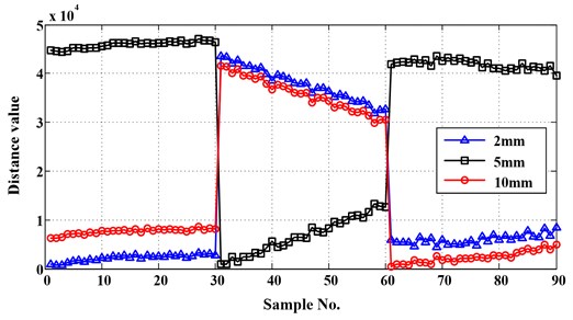
Fig. 15Distances between test samples and reference sets belong to crack
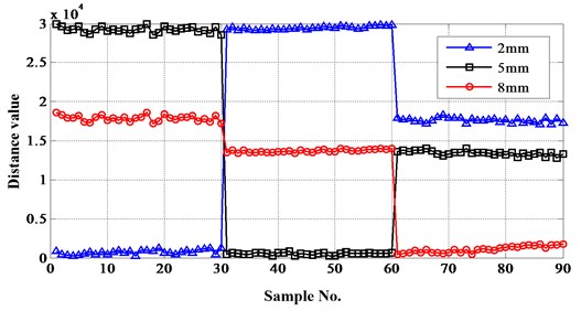
The results show that the proposed approach is also effective to damage level identification. It can classify the different fault lengths of breaktooth and crack accurately. For the case study, the successfully rate of the method using on damage level recognition is 100 %.
4. Industrial data analysis
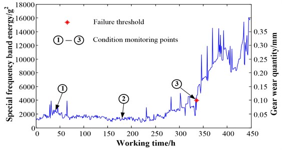
In industrial practical application, the lifetime distribution of mechanical products have particular characteristic. In general, the total lifetime period can be diveded into two stages. And the two stages can be reflected directly by extracting one feature parameter of the vibration signal, as Fig. 16 shows. The figure is the result of extracting special frequency band energy of total lifetime period vibration signal of a gearbox. The vibration signal is acquired from a gearbox total lifetime experiment. The specific explanation about Fig. 16 and the experiment details can be seen in document [22]. In Fig. 16, the axis is the working time, the left axis is the special frequency band energy and the right axis is the gear wear quantity. As a common sense, a product can be continue used even if slight damage happens on it. However, if the damage become severe, maintainence or replacement should implemented to avoid loss. Therefore, people usually take actions to a equipment after using fixed time or one index which obtained from a monitoring instrument exceed a setted failure threshold. And the fixed time or failure threshold often come from practical application of a equipment. As Fig. 16 shows, the special frequency band energy rises rapidly after gear wear quantity exceed 0.10 mm. So, the energy value, 4000, can be select as a failure threshold. Thus, the method proposed in this paper can be a program in a instrument. In order to make the judgement more accurate, some condition monitoring points can be setted. For example, three points are setted as Fig. 16 shows. The first is at the beginning of the equipment operation, the second is in the middle of the first and the third, the third is the failure threshold point. As the flowchart described in Section 2.1, the health condition of the test samples can be judged according to the euclidean distance between the test samples and the trained samples of the three points. Namely, if the distances value between the test samples and the trained samples of the first or second points are the minimum, then the equipment is in normal condition and can be continue used. However, if the distances value between the test samples and the trained samples of the third point are the minimum, then maybe the equipment is in failure condition and need to stop working to be examined and repaired.
Fig. 16Special frequency band energy of total lifetime period vibration signal of a gearbox
On the basis of the viewpoint described above, this paper analyzed the industrial data to validate the effectiveness of the proposed method. And the industrial data was acquired from wind turbines. The type of the wind turbine is FL600 and they are reaching to the examine and repair deadline. The wind turbine gearbox and its internal structure can be seen in Fig. 17.
Fig. 17a) FL600 wind turbine gearbox, b) the internal structure of the gearbox
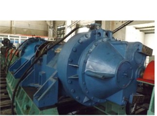
a)
b)
Five acclerometers were utilized to acquire vibration data, as Fig. 17(b) shows. The data acquired from the fourth acclerometer was selected as the test sample due to the planetary structure is the most possible fault component. Three periods data of the historical total lifetime was chosen as the trained sample. And there were three conditions of gearboxes corresponding to the three periods, they are initial, middle and fault conditions. Each condition has 30 trained samples. The results of the proposed method can be seen in Fig. 18. It can be seen from the figure that the Euclidean distances between test samples and the 61-90 trained samples were the minimum. Therefore, the gearbox was in the fault condition.
Fig. 18The results of the proposed method
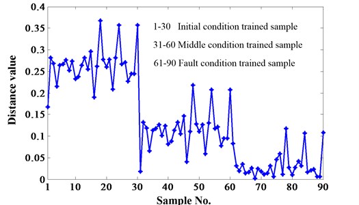
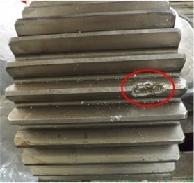
After obtaining the diagnosis result, the gearbox was opened to validate it. The fact proved the diagnosis result was correct, one of the planetary gears was damaged seriously, as Fig. 19 shows. It also proved the effectiveness of the method this paper proposed.
Fig. 19The damaged planetary gear of the wind turbine gearbox
5. Conclusions
In this paper, a novel method based on Hilbert transform (HT) and Euclidean distance technique (EDT) was proposed to classify gear fault modes and identify damage levels for every fault mode. The study was tested and validated successfully in gear monitoring experiment. And the effectiveness of the methodology was demonstrated by the results obtained from the analysis. After contrasted with kurtosis and skewness, energy was selected as the fault feature. Similarly, the approach defined six filters to obtain the energies of the six frequency bands based on the comparation with the energy of the whole signal. HT was used to obtain analytic signal and then EDT was utilized to recognize the different fault modes and levels. Firstly, distinguish the normal condition, breaktooth and crack. Then the damage levels belong to breaktooth and crack were discriminated. Meanwhile, the three cases were all identified with an accurate rate of 100 % which is higher than utilize FDA as comparison. Additionly, industrial data was used to validate the applicability of the proposed method to the practical environment. The results showed that the method this paper proposed still has good performance.
References
-
Ricci R., Pennacchi P. Diagnostics of gear faults based on EMD and automatic selection of intrinsic mode functions. Mechanical Systems and Signal Processing, Vol. 25, Issue 3, 2011, p. 821-838.
-
Loutridis S. J. Damage detection in gear systems using empirical mode decomposition. Engineering Structures, Vol. 26, Issue 12, 2004, p. 1833-1841.
-
Baccarini L. M. R., Silva V. V. R., et al. SVM practical industrial application for mechanical faults diagnostic. Expert Systems with Applications, Vol. 38, Issue 6, 2011, p. 6980-6984.
-
Tang X. L., Zhuang L., Cai J., Li C. B. Multi-fault classification based on support vector machine trained by chaos particle swarm optimization. Knowledge-Based Systems, Vol. 23, Issue 5, 2010, p. 486-490.
-
Li H., Zhang Y. P., Zheng H. Q. Wear detection in gear system using Hilbert-Huang transform. Journal of Mechanical Science and Technology, Vol. 20, Issue 11, 2006, p. 1781-1789.
-
Yen G. G., Leong W. F. Fault classification on vibration data with wavelet based feature selection scheme. Instrumentation, Systems, and Automation Society, Vol. 45, Issue 2, 2006, p. 141-151.
-
Boutros T., Liang M. Detection and diagnosis of bearing and cutting tool faults using hidden Markov models. Mechanical Systems and Signal Processing, Vol. 25, Issue 6, 2011, p. 2012-2124.
-
Kang J. S., Zhang X. H. Application of Hidden Markov Models in machine fault diagnosis. Information – An International Interdispilinary Journal, Vol. 15, Issue 12(B), 2012, p. 5829-5838.
-
Hassiotis S. Identification of damage using natural frequencies and Markov parameters. Computers and Structures, Vol. 74, Issue 3, 2000, p. 365-373.
-
Samuel P. D., Pines D. J. A review of vibration-based techniques for helicopter transmission diagnostics. Journal of Sound and Vibration, Vol. 282, 2005, p. 475-508.
-
Saravanan N., Ramachandran K. I. Fault diagnosis of spur bevel gear box using discrete wavelet features and decision tree classification. Expert Systems with Applications, Vol. 36, Issue 5, 2009, p. 9564-9573.
-
Fan X. F., Zuo M. J. Gearbox fault detection using Hilbert and wavelet packet transform. Mechanical Systems and Signal Processing, Vol. 20, Issue 4, 2006, p. 966-982.
-
Jardine A. K. S., Lin D. M., Banjevic D. A review on machinery diagnostics and prognostics implementing condition-based maintenance. Mechanical Systems and Signal Processing, Vol. 20, 2006, p. 1483-1510.
-
Lebold M., McClintic K., Campbell R., et al. Review of vibration analysis methods for gearbox diagnostics and prognostics. Proceeding of the 54th Meeting of the Society for Machinery Failure Prevention Technology, 2000, p. 623-634.
-
Casimir R., Boutleux E., Clerc G., Yahoui A. The use of features selection and nearest neighbors rule for faults diagnostic in induction motors. Engineering Applications of Artificial Intelligence, Vol. 19, Issue 2, 2006, p. 169-177.
-
Wu J. D., Hsu C. C., Wu G. Z. Fault gear identification and classification using discrete wavelet transform and adaptive neuro-fuzzy inference. Expert Systems with Applications, Vol. 36, Issue 3, 2009, p. 6244-6255.
-
Lei Y. G., Zuo M. J. Gear crack level identification based on weighted K nearest neighbor classification algorithm. Mechanical Systems and Signal Processing, Vol. 23, Issue 5, 2009, p. 1535-1547.
-
Saravanan N., Kumar Siddabattuni V. N. S., Ramachandran K. I. A comparative study on classification of features by SVM and PSVM extracted using Morlet wavelet for fault diagnosis of spur bevel gear box. Expert Systems with Applications, Vol. 35, Issue 3, 2008, p. 1351-1366.
-
Kim K. O., Zuo M. J. Two fault classification methods for large systems when available data are limited. Reliability Engineering and System Safety, Vol. 92, Issue 5, 2007, p. 585-592.
-
Liu Z. L., Qu J., Zuo M. J., Xu H. B. Fault level diagnosis for planetary gearboxes using hybrid kernel feature selection and kernel Fisher discriminant analysis. International Journal of Advanced Manufacturing Technology, Vol. 67, 2013, p. 1217-1230.
-
Du Z. M., Jin X. Q. Multiple faults diagnosis for sensors in air handling unit using Fisher discriminant analysis. Energy Conversion and Management, Vol. 49, 2008, p. 3654-3665.
-
Teng H. Z., Zhao J. M., Jia X. S., et al. Experimental study on gearbox prognosis using total life vibration analysis. Prognostics and System Health Management Conference, Shenzhen, MU3045, 2011.
About this article

