Stability analysis and response of nonlinear rotor-seal system

Sayed, M.; Hamed, Y. S.

Journal of Vibroengineering

Browse Journal

Submit article

Published: 30 December 2014

Check for updates

Stability analysis and response of nonlinear rotor-seal system

M. Sayed¹

Y. S. Hamed²

^{1, 2}Department of Mathematics and Statistics, Faculty of Science, Taif University, El-Taif, El-Haweiah, P.O. Box 888, Zip Code 21974, Kingdom of Saudi Arabia

^{1, 2}Department of Engineering Mathematics, Faculty of Electronic Engineering, Menoufia University, Menouf 32952, Egypt

Corresponding Author:

M. Sayed

Cite the article Download PDF

Downloads 1151

WoS Core Citations 12

Abstract

In this paper, we study the stability of the nonlinear rotor-seal system using Liapunov’s first method. The mathematical solutions using multiple scales up to and including second order approximations is investigated. We extract all resonance cases from analytical solution and investigated. It is quite clear that some of the simultaneous resonance cases are undesirable in the design of such system as they represent some of the worst behavior of the system. The effects of various parameters on the behavior of the system and stability of the system are investigated numerically by response curve. Poincaré maps are used to determine stability and plot bifurcation diagrams.

1. Introduction

Rotating machinery is widely used in engineering. In order to increase the efficiency of rotating machinery, the clearance between rotor and stator has been designed to be smaller and smaller, however, which leads to a larger possibility of impact-rub. Rubbing may induce the rotor’s dynamic instability, blade break, and other serious accidents. Therefore, how to avoid rub and how to reduce the harm caused by rubs become an important problem in rotor dynamics. With the fast development of society and economy, there is a higher demand of improvement in speed, capacity, efficiency and safety reliability in the rotating machinery, such as great power turbo-generator units, shipboard steam turbines, high speed centrifugal compressors, aeroengine and high precision machine. Under some operating conditions, the nonlinear gas exciting force of labyrinth seals in the small gap can cause rotating machines to exhibit whirl-whip instability. Particular, the gas exciting force in ultra supercritical steam turbine unit shows significant influence on the system stability and sometimes can cause disastrous consequences [1].

Up to now, lots of researches have been done. However, the experimental research of gas exciting vibration in steam turbines is hard to proceed. Many researchers have designed the rotor-seal rigs to test the gas exciting force using the similarity theory [2-3]. However, the test accuracy is seriously affected by the testing conditions. In these years, computational fluid dynamics (CFD) and the computer technology have been developed. Recently, many researchers started to use the CFD method to simulate the gas exciting force of the labyrinth seals, and have obtained better results of the dynamic characteristics [4-5]. On the other hand, in 1965, Alford [6] first derived the formula of the gas exciting force when he researched on the stability of aeroengine. Ding and Zhang [7] applied both standard Galerkin method (SGM) and nonlinear Galerkin method (NGM) to numerically investigate the lateral vibration of a continuous rotor system with actions of oil-film force and seal fluid force. Improvement of the NGM procedure over the SGM procedure is discussed and the dynamics of nonlinear rotor system is revealed. Chen et al. [8] utilized the incremental harmonic balance method to obtain the solutions of a rotor-seal system, where the complicated nonlinearities are handled by the expansion method. Periodic, double-periodic and triple-periodic solutions are obtained in excellent agreement with numerical results, which shows the validity and efficacy of the proposed solution procedures.

Li et al. [9] used the Runge–Kutta method to solve the motion equation of the rotor/seal/bearing system. The dynamic characteristics of the rotor/bearing/seal system were analyzed with bifurcation diagrams, time-history diagrams, trajectory diagrams, Poincare maps and frequency spectrums. The numerical analysis indicates that the seal force and the oil-film force influence the nonlinear dynamic characteristics of the rotor system. Zhang and Chen [10] investigated analytically and numerically the full annular rub of a typical nonlinear Jeffcott rotor. Averaging method is used to find the synchronous response of governing equations. Routh-Hurwitz criteria are employed to analyze the stability of synchronous full annular rub solution and determine the boundaries of static and Hopf bifurcations. Finally, the response and onset condition of reverse dry whip are investigated numerically and at the same time, the influences of rotor parameters and rotation speed on the characteristics of the rotor response are investigated. Cheng et al. [11] investigated the non-linear dynamic behaviors of a rotor-bearing-seal coupled system by using Muszynska’s non-linear seal fluid dynamic force model and non-linear oil film force, and the result from the numerical analysis is in agreement with the one from the experiment. The bifurcation of the coupled system is analyzed under different operating conditions. Ding et al. [12] studied Hopf bifurcation and the self-excited vibration with parametric excitation of a single span rotor-seal system, applying the central manifold theorem and normal formal form theory. The results showed that non-synchronized whirl of the imbalanced rotor can either be a quasi-periodic motion resulting from the Hopf bifurcation or a half-frequency whirl from the period doubling bifurcation. Li and Chen [13] investigated the 1:2 sub-harmonic resonance of the labyrinth seals-rotor system, where the low-frequency vibration of steam turbines can be caused by the gas exciting force. The empirical parameters of gas exciting force of the Muszynska model are obtained by using the results of computational fluid dynamics (CFD).

Sayed and Mousa [14] investigated the influence of the quadratic and cubic terms on non-linear dynamic characteristics of the angle-ply composite laminated rectangular plate with parametric and external excitations. The method of multiple time scale perturbation is applied to solve the non-linear differential equations describing the system up to and including the second-order approximation. Two cases of the sub-harmonic resonances cases in the presence of 1:2 internal resonance are considered. The stability of the system is investigated using both frequency response equations and phase-plane method. It is quite clear that some of the simultaneous resonance cases are undesirable in the design of such system as they represent some of the worst behavior of the system. Such cases should be avoided as working conditions for the system. Eissa and Sayed [15-17] and Sayed [18] studied the effects of different active controllers on simple and spring pendulum at the primary resonance via negative velocity feedback or its square or cubic. Amer et al. [19] studied the dynamical system of a twin-tail aircraft, which is described by two coupled second order nonlinear differential equations having both quadratic and cubic nonlinearities, solved and controlled. The system is subjected to both multi-parametric and multi-external excitations. The method of multiple time scale perturbation is applied to solve the nonlinear differential equations up to the two order approximations. The stability of the system is investigated applying both frequency response equations and phase plane method. Two simple active control laws based on the linear negative velocity and acceleration feedback are used. Sayed and Hamed [20] studied the response of a two-degree-of-freedom system with quadratic coupling under parametric and harmonic excitations. The method of multiple scale perturbation technique is applied to solve the non-linear differential equations and obtain approximate solutions up to and including the second-order approximations.

Hamed et al. [21-23] studied USM model subject to multi-external or both multi-external and multi-parametric and both multi-external and tuned excitation forces. The model consists of multi-degree-of-freedom system consisting of the tool holder and absorbers (tools) simulating ultrasonic machining process. The advantages of using multi-tools are to machine different materials and different shapes at the same time. This leads to time saving and higher machining efficiency. Hamed et al. [24] presented the behavior of the nonlinear string beam coupled system subjected to external, parametric and tuned excitations for case 1:1 internal resonance. The stability of the system studied using frequency response equations and phase-plane method. It is found from numerical simulations that there are obvious jumping phenomena in the frequency response curves. Sayed and Kamel [25, 26] investigated the effect of different controllers on the vibrating system and the saturation control of a linear absorber to reduce vibrations due to rotor blade flapping motion. The stability of the obtained numerical solution is investigated using both phase plane methods and frequency response equations. Sayed et al. [27] investigated the non-linear dynamics of a two-degree-of freedom vibration system including quadratic and cubic non-linearities subjected to external and parametric excitation forces. There exist multi-valued solutions which increase or decrease by the variation of some parameters. The numerical simulations show the system exhibits periodic motions and chaotic motions. Sayed and Mousa [28] studied an analytical investigation of the nonlinear vibration of a symmetric cross-ply composite laminated piezoelectric rectangular plate under parametric and external excitations. Their study focused on the case of 1:1:3 primary resonance and internal resonance, and they verified the analytical results calculated by the method of multiple time scale by comparing them with the numerical results of the modal equations. The obtained results were verified by comparing the results of the finite difference method (FDM) and Runge-Kutta (RKM) method. When plotting the solutions to some nonlinear problems, the phase space can become overcrowded and the underlying structure may become obscured. To overcome these difficulties, a basic tool of Poincaré maps was proposed by Henri Poincaré [29] at the end of the nineteenth century.

2. Model of rotor-seal system

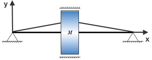
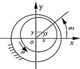
Assume that such an anisotropic rotor mounts at both rigid ends and rotates in the gas seals, and its rotation causes gas rotation and subsequently generates the gas exciting force. Suppose that the external force has a rotating character with synchronous frequencies due to the rotor unbalance. The mathematical model of the rotor-seal system in the stationary reference coordinates ( $x$ , $y$ ) as shown in Fig. 1 can be deduced as [13]:

1

(\begin{matrix} M + m & 0 \\ 0 & M + m \end{matrix}) (\begin{matrix} \ddot{x} \\ \ddot{y} \end{matrix}) + (\begin{matrix} D_{x e} + D & 2 m λ Ω \\ - 2 m λ Ω & D_{y e} + D \end{matrix}) (\begin{matrix} \dot{x} \\ \dot{y} \end{matrix})

+ (\begin{matrix} K_{x e} + K - m λ^{2} Ω^{2} & λ Ω D \\ - λ Ω D & K_{y e} + K - m λ^{2} Ω^{2} \end{matrix}) (\begin{matrix} x \\ y \end{matrix}) = (\begin{matrix} ρ \cos (Ω t) \\ G + ρ \sin (Ω t) \end{matrix}),

where $M$ is the rotor mass, $m$ is the gas inertia effects, $K_{x e}$ , $K_{y e}$ , $D_{x e}$ , $D_{y e}$ are the stiffness and external damping on the $x$ and $y$ directions respectively and $G$ is the gravitation effects of the rotor, $ρ$ is the amplitude of the excitation force.

Fig. 1Model of rotor-seal system

a)

b)

3. Mathematical analysis

The motion equation of a rotor-seal system (1) can be obtained by:

2a

\ddot{x} + ω_{1}^{2} x = f_{x} (x, y, \dot{x}, \dot{y}) + ρ c o s (Ω t),

2b

\ddot{y} + ω_{2}^{2} y = f_{y} (x, y, \dot{x}, \dot{y}) + ρ s i n (Ω t),

with initial condition $x (0) = \dot{x} (0) = y (0) = \dot{y} (0) = 0$ . Where $x$ and $y$ are the displacements of the shaft center, $ω_{1}$ and $ω_{2}$ the linear natural frequencies in $x$ , $y$ directions, and $Ω$ the angular speed of the rotor, $ρ$ is the amplitude of the excitation force, $f_{x} (x, y, \dot{x}, \dot{y})$ and $f_{y} (x, y, \dot{x}, \dot{y})$ are power series function of the nonlinear force on $x$ and $y$ directions given by:

f_{x} (x, y, \dot{x}, \dot{y}) = α_{1} x + α_{2} \dot{x} + α_{3} y + α_{4} \dot{y} + α_{5} x^{2} + α_{6} y^{2} + α_{7} x \dot{x} + α_{8} x y + α_{9} x \dot{y}

+ α_{10} \dot{x} y + α_{11} y \dot{y} + α_{12} x^{3} + α_{13} y^{3} + α_{14} x^{2} \dot{x} + α_{15} x^{2} y + α_{16} x^{2} \dot{y} + α_{17} x y^{2}

+ α_{18} y^{2} \dot{x} + α_{19} y^{2} \dot{y} + α_{20} x y \dot{x} + α_{21} x y \dot{y},

f_{y} (x, y, \dot{x}, \dot{y}) = β_{1} x + β_{2} \dot{x} + β_{3} y + β_{4} \dot{y} + β_{5} x^{2} + β_{6} y^{2} + β_{7} x \dot{x} + β_{8} x y + β_{9} x \dot{y}

+ β_{10} \dot{x} y + β_{11} y \dot{y} + β_{12} x^{3} + β_{13} y^{3} + β_{14} x^{2} \dot{x} + β_{15} x^{2} y + β_{16} x^{2} \dot{y} + β_{17} x y^{2}

+ β_{18} y^{2} \dot{x} + β_{19} y^{2} \dot{y} + β_{20} x y \dot{x} + β_{21} x y \dot{y}

All coefficient of $α_{i}$ , $β_{i}$ are defined in [13]. The linear, non-linear coefficients and excitation amplitude are assumed to be:

3

α_{n} = ε {\hat{α}}_{n}, β_{n} = ε {\hat{β}}_{n}, ρ = ε \hat{ρ}, n = 1, 2, . . ., 21,

where $ε$ is a small perturbation parameter and $0 < ε < < 1$ .

To consider the influence of the quadratic and cubic terms on non-linear dynamic characteristics of the non-linear rotor-seal system, we need to obtain the second-order approximate solution of Eqs. (2). We determine a second-order approximation for the system response by the method of multiple scales [30-31], which is a powerful tool in determining periodic solutions of small amplitude. For the second-order approximation, introducing three time scales:

4

T_{n} = ε^{n} t, n = 0, 1, 2 .

We seek an asymptotic solution of Eqs. (2) for $x$ and $y$ in the form of:

5

x (t, ε) = x_{0} (T_{0}, T_{1}, T_{2}) + ε x_{1} (T_{0}, T_{1}, T_{2}) + ε^{2} x_{2} (T_{0}, T_{1}, T_{2}) + O (ε^{3}),

6

y (t, ε) = y_{0} (T_{0}, T_{1}, T_{2}) + ε y_{1} (T_{0}, T_{1}, T_{2}) + ε^{2} y_{2} (T_{0}, T_{1}, T_{2}) + O (ε^{3}) .

Derivatives with respect to $t$ are then transformed into:

7

\frac{d}{d t} = \frac{\partial}{\partial T_{0}} \frac{\partial T_{0}}{\partial t} + \frac{\partial}{\partial T_{1}} \frac{\partial T_{1}}{\partial t} + \frac{\partial}{\partial T_{2}} \frac{\partial T_{2}}{\partial t} = D_{0} + ε D_{1} + ε^{2} D_{2},

8

\frac{d^{2}}{d t^{2}} = D_{0}^{2} + 2 ε D_{0} D_{1} + ε^{2} (D_{1}^{2} + 2 D_{0} D_{2}),

where $D_{n} = \partial / \partial T_{n}$ , $n =$ 0, 1, 2. Terms of $O (ε^{3})$ and higher orders are neglected. Substituting Eqs. (5)-(6) and (7)-(8) into Eqs. (2) and equating the coefficients of similar powers of $ε$ , one obtains the following set of ordinary differential equations:

Order $ε^{0}$ :

9

(D_{0}^{2} + ω_{1}^{2}) x_{0} = 0,

10

(D_{0}^{2} + ω_{2}^{2}) y_{0} = 0 .

Order $ε^{1}$ :

11

(D_{0}^{2} + ω_{1}^{2}) x_{1} = - 2 D_{0} D_{1} x_{0} + {\hat{α}}_{1} x_{0} + {\hat{α}}_{2} D_{0} x_{0} + {\hat{α}}_{3} y_{0} + {\hat{α}}_{4} D_{0} y_{0} + {\hat{α}}_{5} x_{0}^{2} + {\hat{α}}_{6} y_{0}^{2}

+ {\hat{α}}_{7} x_{0} D_{0} x_{0} + {\hat{α}}_{8} x_{0} y_{0} + {\hat{α}}_{9} x_{0} D_{0} y_{0} + {\hat{α}}_{10} y_{0} D_{0} x_{0} + {\hat{α}}_{11} y_{0} D_{0} y_{0} + {\hat{α}}_{12} x_{0}^{3} + {\hat{α}}_{13} y_{0}^{3}

+ {\hat{α}}_{14} x_{0}^{2} D_{0} x_{0} + {\hat{α}}_{15} x_{0}^{2} y_{0} + {\hat{α}}_{16} x_{0}^{2} D_{0} y_{0} + {\hat{α}}_{17} x_{0} y_{0}^{2} + {\hat{α}}_{18} y_{0}^{2} D_{0} x_{0} + {\hat{α}}_{19} y_{0}^{2} D_{0} y_{0}

+ {\hat{α}}_{20} x_{0} y_{0} D_{0} x_{0} + {\hat{α}}_{21} x_{0} y_{0} D_{0} y_{0} + \hat{ρ} c o s (Ω t),

12

(D_{0}^{2} + ω_{2}^{2}) y_{1} = - 2 D_{0} D_{1} y_{0} + {\hat{β}}_{1} x_{0} + {\hat{β}}_{2} D_{0} x_{0} + {\hat{β}}_{3} y_{0} + {\hat{β}}_{4} D_{0} y_{0} + {\hat{β}}_{5} x_{0}^{2} + {\hat{β}}_{6} y_{0}^{2}

+ {\hat{β}}_{7} x_{0} D_{0} x_{0} + {\hat{β}}_{8} x_{0} y_{0} + {\hat{β}}_{9} x_{0} D_{0} y_{0} + {\hat{β}}_{10} y_{0} D_{0} x_{0} + {\hat{β}}_{11} y_{0} D_{0} y_{0} + {\hat{β}}_{12} x_{0}^{3} + {\hat{β}}_{13} y_{0}^{3}

+ {\hat{β}}_{14} x_{0}^{2} D_{0} x_{0} + {\hat{β}}_{15} x_{0}^{2} y_{0} + {\hat{β}}_{16} x_{0}^{2} D_{0} y_{0} + {\hat{β}}_{17} x_{0} y_{0}^{2} + {\hat{β}}_{18} y_{0}^{2} D_{0} x_{0} + {\hat{β}}_{19} y_{0}^{2} D_{0} y_{0}

+ {\hat{β}}_{20} x_{0} y_{0} D_{0} x_{0} + {\hat{β}}_{21} x_{0} y_{0} D_{0} y_{0} + \hat{ρ} s i n (Ω t) .

Order $ε^{2}$ :

13

(D_{0}^{2} + ω_{1}^{2}) x_{2} = - D_{1}^{2} x_{1} - 2 D_{0} D_{2} x_{0} - 2 D_{0} D_{1} x_{1} + {\hat{α}}_{1} x_{1} + {\hat{α}}_{2} (D_{0} x_{1} + D_{1} x_{0}) + {\hat{α}}_{3} y_{1}

+ {\hat{α}}_{4} (D_{0} y_{1} + D_{1} y_{0}) + 2 {\hat{α}}_{5} x_{0} x_{1} + 2 {\hat{α}}_{6} y_{0} y_{1} + {\hat{α}}_{7} x_{1} D_{0} x_{0} + {\hat{α}}_{7} x_{0} (D_{0} x_{1} + D_{1} x_{0})

+ {\hat{α}}_{8} (x_{0} y_{1} + x_{1} y_{0}) + {\hat{α}}_{9} x_{1} D_{0} y_{0} + {\hat{α}}_{9} x_{0} (D_{0} y_{1} + D_{1} y_{0}) + {\hat{α}}_{10} y_{1} D_{0} x_{0}

+ {\hat{α}}_{10} y_{0} (D_{0} x_{1} + D_{1} x_{0}) + {\hat{α}}_{11} y_{1} D_{0} y_{0} + {\hat{α}}_{11} y_{0} (D_{0} y_{1} + D_{1} y_{0}) + 3 {\hat{α}}_{12} x_{0}^{2} x_{1}

+ 3 {\hat{α}}_{13} y_{0}^{2} y_{1} + 2 {\hat{α}}_{14} x_{0} x_{1} D_{0} x_{0} + {\hat{α}}_{14} x_{0}^{2} (D_{0} x_{1} + D_{1} x_{0}) + {\hat{α}}_{15} x_{0}^{2} y_{1} + 2 {\hat{α}}_{15} x_{0} y_{0} x_{1}

+ 2 {\hat{α}}_{16} x_{0} x_{1} D_{0} y_{0} + {\hat{α}}_{16} x_{0}^{2} (D_{0} y_{1} + D_{1} y_{0}) + 2 {\hat{α}}_{17} y_{0} y_{1} x_{0} + {\hat{α}}_{17} y_{0}^{2} x_{1} + 2 {\hat{α}}_{18} y_{0} y_{1} D_{0} x_{0}

+ {\hat{α}}_{18} y_{0}^{2} (D_{0} x_{1} + D_{1} x_{0}) + {\hat{α}}_{19} y_{0}^{2} (D_{0} y_{1} + D_{1} y_{0}) + 2 {\hat{α}}_{19} y_{0} y_{1} D_{0} y_{0}

+ {\hat{α}}_{20} x_{0} y_{0} (D_{0} x_{1} + D_{1} x_{0}) + ({\hat{α}}_{20} x_{0} y_{1} + {\hat{α}}_{20} x_{1} y_{0}) D_{0} x_{0} + {\hat{α}}_{21} x_{0} y_{0} (D_{0} y_{1} + D_{1} y_{0})

+ ({\hat{α}}_{21} x_{0} y_{1} + {\hat{α}}_{21} x_{1} y_{0}) D_{0} y_{0},

14

(D_{0}^{2} + ω_{2}^{2}) y_{2} = - D_{1}^{2} y_{1} - 2 D_{0} D_{2} y_{0} - 2 D_{0} D_{1} y_{1} + {\hat{β}}_{1} x_{1} + {\hat{β}}_{2} (D_{0} x_{1} + D_{1} x_{0}) + {\hat{β}}_{3} y_{1}

+ {\hat{β}}_{4} (D_{0} y_{1} + D_{1} y_{0}) + 2 {\hat{β}}_{5} x_{0} x_{1} + 2 {\hat{β}}_{6} y_{0} y_{1} + {\hat{β}}_{7} x_{1} D_{0} x_{0} + {\hat{β}}_{7} x_{0} (D_{0} x_{1} + D_{1} x_{0})

+ {\hat{β}}_{8} (x_{0} y_{1} + x_{1} y_{0}) + {\hat{β}}_{9} x_{1} D_{0} y_{0} + {\hat{β}}_{9} x_{0} (D_{0} y_{1} + D_{1} y_{0}) + {\hat{β}}_{10} y_{1} D_{0} x_{0}

+ {\hat{β}}_{10} y_{0} (D_{0} x_{1} + D_{1} x_{0}) + {\hat{β}}_{11} y_{1} D_{0} y_{0} + {\hat{β}}_{11} y_{0} (D_{0} y_{1} + D_{1} y_{0}) + 3 {\hat{β}}_{12} x_{0}^{2} x_{1}

+ 3 {\hat{β}}_{13} y_{0}^{2} y_{1} + 2 {\hat{β}}_{14} x_{0} x_{1} D_{0} x_{0} + {\hat{β}}_{14} x_{0}^{2} (D_{0} x_{1} + D_{1} x_{0}) + {\hat{β}}_{15} x_{0}^{2} y_{1} + 2 {\hat{β}}_{15} x_{0} y_{0} x_{1}

+ 2 {\hat{β}}_{16} x_{0} x_{1} D_{0} y_{0} + {\hat{β}}_{16} x_{0}^{2} (D_{0} y_{1} + D_{1} y_{0}) + 2 {\hat{β}}_{17} y_{0} y_{1} x_{0} + {\hat{β}}_{17} y_{0}^{2} x_{1} + 2 {\hat{β}}_{18} y_{0} y_{1} D_{0} x_{0}

+ {\hat{β}}_{18} y_{0}^{2} (D_{0} x_{1} + D_{1} x_{0}) + {\hat{β}}_{19} y_{0}^{2} (D_{0} y_{1} + D_{1} y_{0}) + 2 {\hat{β}}_{19} y_{0} y_{1} D_{0} y_{0}

+ {\hat{β}}_{20} x_{0} y_{0} (D_{0} x_{1} + D_{1} x_{0}) + ({\hat{β}}_{20} x_{0} y_{1} + {\hat{β}}_{20} x_{1} y_{0}) D_{0} x_{0} + {\hat{β}}_{21} x_{0} y_{0} (D_{0} y_{1} + D_{1} y_{0})

+ ({\hat{β}}_{21} x_{0} y_{1} + {\hat{β}}_{21} x_{1} y_{0}) D_{0} y_{0} .

The general solutions of Eqs. (9)-(10), can be written in the form:

15

x_{0} = A_{1} (T_{1}, T_{2}) e x p (i ω_{1} T_{0}) + c c,

16

y_{0} = A_{2} (T_{1}, T_{2}) e x p (i ω_{2} T_{0}) + c c,

where $A_{1}$ and $A_{2}$ are a complex function in $T_{1}$ , $T_{2}$ and $c c$ indicates the complex conjugates of the preceding terms. Substituting Eqs. (15)-(16) into Eqs. (11)-(12) and after eliminating the secular terms, the non-homogeneous solutions of Eqs. (11)-(12) are:

17

x_{1} = E_{1} e x p (2 i ω_{1} T_{0}) + E_{2} e x p (3 i ω_{1} T_{0}) + E_{3} e x p (i ω_{2} T_{0}) + E_{4} e x p (2 i ω_{2} T_{0})

+ E_{5} e x p (3 i ω_{2} T_{0}) + E_{6} e x p (i (ω_{1} \pm ω_{2}) T_{0}) + E_{7} e x p (i (ω_{1} \pm 2 ω_{2}) T_{0})

+ E_{8} e x p (i (2 ω_{1} \pm ω_{2}) T_{0}) + E_{9} e x p (i Ω T_{0}) + E_{10} + c c,

18

y_{1} = E_{11} e x p (i ω_{1} T_{0}) + E_{12} e x p (2 i ω_{1} T_{0}) + E_{13} e x p (3 i ω_{1} T_{0}) + E_{14} e x p (2 i ω_{2} T_{0})

+ E_{15} e x p (3 i ω_{2} T_{0}) + E_{16} e x p (i (ω_{1} \pm ω_{2}) T_{0}) + E_{17} e x p (i (ω_{1} \pm 2 ω_{2}) T_{0})

+ E_{18} e x p (i (2 ω_{1} \pm ω_{2}) T_{0}) + E_{19} e x p (i Ω T_{0}) + E_{20} + c c,

where $E_{i}$ ( $i = 1, 2, ..., 20$ ) are complex functions in $T_{1}$ and $T_{2}$ . Substituting Eqs. (15)-(18) into Eqs. (13)-(14) and after eliminating the secular terms, the non-homogeneous solutions of Eqs. (13)-(14) are:

19

x_{2} = H_{1} e x p (2 i ω_{1} T_{0}) + H_{2} e x p (3 i ω_{1} T_{0}) + H_{3} e x p (4 i ω_{1} T_{0}) + H_{4} e x p (5 i ω_{1} T_{0})

+ H_{5} e x p (i ω_{2} T_{0}) + H_{6} e x p (2 i ω_{2} T_{0}) + H_{7} e x p (3 i ω_{2} T_{0}) + H_{8} e x p (4 i ω_{2} T_{0})

+ H_{9} e x p (5 i ω_{2} T_{0}) + H_{10} e x p (i (ω_{1} \pm ω_{2}) T_{0}) + H_{11} e x p (i (ω_{1} \pm 2 ω_{2}) T_{0})

+ H_{12} e x p (i (2 ω_{1} \pm ω_{2}) T_{0}) + H_{13} e x p (i (2 ω_{1} \pm 2 ω_{2}) T_{0}) + H_{14} e x p (i (ω_{1} \pm 3 ω_{2}) T_{0})

+ H_{15} e x p (i (ω_{1} \pm 4 ω_{2}) T_{0}) + H_{16} e x p (i (2 ω_{1} \pm 3 ω_{2}) T_{0}) + H_{17} e x p (i (3 ω_{1} \pm 2 ω_{2}) T_{0})

+ H_{18} e x p (i (3 ω_{1} \pm ω_{2}) T_{0}) + H_{19} e x p (i (4 ω_{1} \pm ω_{2}) T_{0}) + H_{20} e x p (i Ω T_{0})

+ H_{21} e x p (2 i Ω T_{0}) + H_{22} e x p (3 i Ω T_{0}) + H_{23} e x p (4 i Ω T_{0}) + H_{24} e x p (5 i Ω T_{0})

+ H_{25} e x p (i (ω_{1} \pm Ω) T_{0}) + H_{26} e x p (i (2 ω_{1} \pm Ω) T_{0}) + H_{27} e x p (i (ω_{1} \pm 2 Ω) T_{0})

+ H_{28} e x p (i (ω_{1} \pm 3 Ω) T_{0}) + H_{29} e x p (i (ω_{1} \pm 4 Ω) T_{0}) + H_{30} e x p (i (2 ω_{1} \pm 2 Ω) T_{0})

+ H_{31} e x p (i (2 ω_{1} \pm 3 Ω) T_{0}) + H_{32} e x p (i (3 ω_{1} \pm Ω) T_{0}) + H_{33} e x p (i (3 ω_{1} \pm 2 Ω) T_{0})

+ H_{34} e x p (i (4 ω_{1} \pm Ω) T_{0}) + H_{35} e x p (i (ω_{2} \pm Ω) T_{0}) + H_{36} e x p (i (2 ω_{2} \pm Ω) T_{0})

+ H_{37} e x p (i (ω_{2} \pm 2 Ω) T_{0}) + H_{38} e x p (i (2 ω_{2} \pm 2 Ω) T_{0}) + H_{39} e x p (i (2 ω_{2} \pm 3 Ω) T_{0})

+ H_{40} e x p (i (ω_{2} \pm 3 Ω) T_{0}) + H_{41} e x p (i (ω_{2} \pm 4 Ω) T_{0}) + H_{42} e x p (i (3 ω_{2} \pm 2 Ω) T_{0})

+ H_{43} e x p (i (3 ω_{2} \pm Ω) T_{0}) + H_{44} e x p (i (4 ω_{2} \pm Ω) T_{0}) + H_{45} e x p (i (2 ω_{1} \pm ω_{2} \pm Ω) T_{0})

+ H_{46} e x p (i (ω_{1} \pm ω_{2} \pm Ω) T_{0}) + H_{47} e x p (i (ω_{1} \pm ω_{2} \pm 2 Ω) T_{0})

+ H_{48} e x p (i (3 ω_{1} \pm ω_{2} \pm Ω) T_{0}) + H_{49} e x p (i (ω_{1} \pm 3 ω_{2} \pm Ω) T_{0})

+ H_{50} e x p (i (ω_{1} \pm ω_{2} \pm 3 Ω) T_{0}) Ω) T_{0}) + H_{51} e x p (i (2 ω_{1} \pm 2 ω_{2} \pm Ω) T_{0})

+ H_{52} e x p (i (2 ω_{1} \pm ω_{2} \pm 2 Ω) T_{0}) + H_{53} e x p (i (ω_{1} \pm 2 ω_{2} \pm 2 Ω) T_{0}) + H_{54} + c c,

20

y_{2} = G_{1} e x p (i ω_{1} T_{0}) + G_{2} e x p (2 i ω_{1} T_{0}) + G_{3} e x p (3 i ω_{1} T_{0}) + G_{4} e x p (4 i ω_{1} T_{0})

+ G_{5} e x p (5 i ω_{1} T_{0}) + G_{6} e x p (2 i ω_{2} T_{0}) + G_{7} e x p (3 i ω_{2} T_{0}) + G_{8} e x p (4 i ω_{2} T_{0})

+ G_{9} e x p (5 i ω_{2} T_{0}) + G_{10} e x p (i (ω_{1} \pm ω_{2}) T_{0}) + G_{11} e x p (i (ω_{1} \pm 2 ω_{2}) T_{0})

+ G_{12} e x p (i (2 ω_{1} \pm ω_{2}) T_{0}) + G_{13} e x p (i (2 ω_{1} \pm 2 ω_{2}) T_{0}) + G_{14} e x p (i (ω_{1} \pm 3 ω_{2}) T_{0})

+ G_{15} e x p (i (ω_{1} \pm 4 ω_{2}) T_{0}) + G_{16} e x p (i (2 ω_{1} \pm 3 ω_{2}) T_{0}) + G_{17} e x p (i (3 ω_{1} \pm 2 ω_{2}) T_{0})

+ G_{18} e x p (i (3 ω_{1} \pm ω_{2}) T_{0}) + G_{19} e x p (i (4 ω_{1} \pm ω_{2}) T_{0}) + G_{20} e x p (i Ω T_{0})

+ G_{21} e x p (2 i Ω T_{0}) + G_{22} e x p (3 i Ω T_{0}) + G_{23} e x p (4 i Ω T_{0}) + G_{24} e x p (5 i Ω T_{0})

+ G_{25} e x p (i (ω_{1} \pm Ω) T_{0}) + G_{26} e x p (i (2 ω_{1} \pm Ω) T_{0}) + G_{27} e x p (i (ω_{1} \pm 2 Ω) T_{0})

+ G_{28} e x p (i (ω_{1} \pm 3 Ω) T_{0}) + G_{29} e x p (i (ω_{1} \pm 4 Ω) T_{0}) + G_{30} e x p (i (2 ω_{1} \pm 2 Ω) T_{0})

+ G_{31} e x p (i (2 ω_{1} \pm 3 Ω) T_{0}) + G_{32} e x p (i (3 ω_{1} \pm Ω) T_{0}) + G_{33} e x p (i (3 ω_{1} \pm 2 Ω) T_{0})

+ G_{34} e x p (i (4 ω_{1} \pm Ω) T_{0}) + G_{35} e x p (i (ω_{2} \pm Ω) T_{0}) + G_{36} e x p (i (2 ω_{2} \pm Ω) T_{0})

+ G_{37} e x p (i (ω_{2} \pm 2 Ω) T_{0}) + G_{38} e x p (i (2 ω_{2} \pm 2 Ω) T_{0}) + G_{39} e x p (i (2 ω_{2} \pm 3 Ω) T_{0})

+ G_{40} e x p (i (ω_{2} \pm 3 Ω) T_{0}) + G_{41} e x p (i (ω_{2} \pm 4 Ω) T_{0}) + G_{42} e x p (i (3 ω_{2} \pm 2 Ω) T_{0})

+ G_{43} e x p (i (3 ω_{2} \pm Ω) T_{0}) + G_{44} e x p (i (4 ω_{2} \pm Ω) T_{0}) + G_{45} e x p (i (2 ω_{1} \pm ω_{2} \pm Ω) T_{0})

+ G_{46} e x p (i (ω_{1} \pm ω_{2} \pm Ω) T_{0}) + G_{47} e x p (i (ω_{1} \pm ω_{2} \pm 2 Ω) T_{0})

+ G_{48} e x p (i (3 ω_{1} \pm ω_{2} \pm Ω) T_{0}) + G_{49} e x p (i (ω_{1} \pm 3 ω_{2} \pm Ω) T_{0})

+ G_{50} e x p (i (ω_{1} \pm ω_{2} \pm 3 Ω) T_{0}) Ω) T_{0}) + G_{51} e x p (i (2 ω_{1} \pm 2 ω_{2} \pm Ω) T_{0})

+ G_{52} e x p (i (2 ω_{1} \pm ω_{2} \pm 2 Ω) T_{0}) + G_{53} e x p (i (ω_{1} \pm 2 ω_{2} \pm 2 Ω) T_{0}) + G_{54} + c c,

where $H_{i}$ , $G_{i}$ ( $i = 1, 2, ..., 54$ ) are complex functions in $T_{1}$ and $T_{2}$ . From the above derived solutions, the reported resonance cases are:

• Primary resonance: $Ω ≅ ω_{n}$ , $n = 1, 2$ .

• Sub-harmonic resonance: $Ω ≅ {k ω}_{n}$ , $k =$ 2, 3, 4, 5 and $n = 1, 2$ .

• Super-harmonic resonance: $k Ω ≅ ω_{n}$ , $3 Ω ≅ {2 ω}_{n}$ , $2 Ω ≅ 3 ω_{n}$ , $k =$ 2, 3, 4, 5 and $n = 1, 2$ .

Internal or secondary resonance: $ω_{1} ≅ s ω_{2}$ , $ω_{2} ≅ s ω_{1}$ , $2 ω_{1} ≅ 3 ω_{2}$ , $3 ω_{1} ≅ 2 ω_{2} s =$ 2, 3, 4, 5.

• Combined resonance: $ω_{1} ≅ \pm m ω_{2} \pm Ω,$ $ω_{1} ≅ \pm ω_{2} \pm r Ω,$ $ω_{1} ≅ \pm 2 ω_{2} \pm 2 Ω,$ $ω_{1} ≅ \pm 2 ω_{2} \pm 3 Ω,$ $ω_{1} ≅ \pm 3 ω_{2} \pm 2 Ω,$ $2 ω_{1} ≅ \pm q ω_{2} \pm Ω,$ $2 ω_{1} ≅ \pm ω_{2} \pm p Ω,$ $3 ω_{1} ≅ \pm n ω_{2} \pm Ω,$ $3 ω_{1} ≅ \pm ω_{2} \pm 2 Ω,$ $4 ω_{1} ≅ \pm ω_{2} \pm Ω,$ $m =$ 1, 2, 3, 4, $r =$ 2, 3, 4, $q =$ 1, 2, 3, $p =$ 2, 3, $n = 1, 2$ .

• Simultaneous or incident resonance.

Any combination of the above resonance cases is considered as simultaneous resonance.

4. Stability analysis

To describe quantitatively the closeness of the resonances, we introduce the detuning parameters $σ_{1}$ and $σ_{2}$ according to:

21

Ω = ω_{1} + ε σ_{1}, ω_{2} = 3 ω_{1} + ε σ_{2} .

Substituting Eq. (21) into Eqs. (11)-(12) and eliminating the secular and small divisor terms from $x_{1}$ and $y_{1}$ , we get the following:

22

2 i ω_{1} D_{1} A = ({\hat{α}}_{1} + i {\hat{α}}_{2} ω_{1}) A + [2 i {\hat{α}}_{18} ω_{1} + 2 {\hat{α}}_{17}] B \bar{B} A

+ [{\hat{α}}_{15} + i {\hat{α}}_{16} ω_{2} - i {\hat{α}}_{20} ω_{1}] {\bar{A}}^{2} B e x p (i σ_{2} T_{1}) + [3 {\hat{α}}_{12} + i {\hat{α}}_{14} ω_{1}] A^{2} \bar{A} + \frac{\hat{ρ}}{2} e x p (i σ_{1} T_{1}),

23

2 i ω_{2} D_{1} B = ({\hat{β}}_{3} + i {\hat{β}}_{4} ω_{2}) B + [3 {\hat{β}}_{13} + i {\hat{β}}_{19} ω_{2}] B^{2} \bar{B}

+ [2 {\hat{β}}_{15} + 2 i {\hat{β}}_{16} ω_{2}] A \bar{A} B + [{\hat{β}}_{12} + i {\hat{β}}_{14} ω_{1}] A^{3} e x p (- i σ_{2} T_{1}) .

To analyze the solution of Eqs. (22)-(23), it is convenient to express the $A (T_{1})$ and $B (T_{1})$ in the polar form as:

24

A (T_{1}) = \frac{1}{2} a (T_{1}) e^{(i γ_{1} (T_{1}))}, B (T_{1}) = \frac{1}{2} b (T_{1}) e^{(i γ_{2} (T_{1}))},

where $a$ , $b$ , $γ_{1}$ and $γ_{2}$ are unknown real-valued functions. Inserting Eq. (24) into Eqs. (22)-(23) and separating real and imaginary parts, we have:

25

a^{'} = \frac{α_{2}}{2} a + \frac{α_{14}}{8} a^{3} + \frac{α_{18}}{4} a b^{2} + \frac{α_{15}}{8 ω_{1}} a^{2} b s i n θ_{2} + (\frac{α_{16} ω_{2} - α_{20} ω_{1}}{8 ω_{1}}) a^{2} b c o s θ_{2}

+ \frac{ρ}{2 ω_{1}} s i n θ_{1},

26

a γ_{1}^{'} = - \frac{α_{1}}{2 ω_{1}} a - \frac{3 α_{12}}{8 ω_{1}} a^{3} - \frac{α_{17}}{4 ω_{1}} a b^{2} - \frac{α_{15}}{8 ω_{1}} a^{2} b c o s θ_{2} + (\frac{α_{16} ω_{2} - α_{20} ω_{1}}{8 ω_{1}}) a^{2} b s i n θ_{2}

- \frac{ρ}{2 ω_{1}} c o s θ_{1},

27

b^{'} = \frac{β_{4}}{2} b + \frac{β_{19}}{8} b^{3} + \frac{β_{16}}{4} a^{2} b - \frac{β_{12}}{8 ω_{2}} a^{3} s i n θ_{2} + \frac{β_{14} ω_{1}}{8 ω_{2}} a^{3} c o s θ_{2},

28

b γ_{2}^{'} = - \frac{β_{3}}{2 ω_{2}} b - \frac{3 β_{13}}{8 ω_{2}} b^{3} - \frac{β_{15}}{4 ω_{2}} a^{2} b - \frac{β_{12}}{8 ω_{2}} a^{3} c o s θ_{2} - \frac{β_{14} ω_{1}}{8 ω_{2}} a^{3} s i n θ_{2},

where:

29

θ_{1} = σ_{1} T_{1} - γ_{1}, θ_{2} = σ_{2} T_{1} + γ_{2} - 3 γ_{1} .

Then, it follows from Eq. (29) that:

30

γ_{1}^{'} = σ_{1} - θ_{1}^{'},

31

γ_{2}^{'} = 3 σ_{1} - σ_{2} + θ_{2}^{'} - 3 θ_{1}^{'} .

The control strategy is evaluated by analyzing the steady state response of the closed-loop system. Setting $a^{'} = b^{'} = 0$ and $θ_{m}^{'} = 0$ ( $m =$ 1, 2) into Eqs. (25)-(28) we obtained:

32

\frac{α_{2}}{2} a + \frac{α_{14}}{8} a^{3} + \frac{α_{18}}{4} a b^{2} + \frac{α_{15}}{8 ω_{1}} a^{2} b s i n θ_{2}

+ (\frac{α_{16} ω_{2} - α_{20} ω_{1}}{8 ω_{1}}) a^{2} b c o s θ_{2} + \frac{ρ}{2 ω_{1}} s i n θ_{1} = 0,

33

a σ_{1} + \frac{α_{1}}{2 ω_{1}} a + \frac{3 α_{12}}{8 ω_{1}} a^{3} + \frac{α_{17}}{4 ω_{1}} a b^{2} + \frac{α_{15}}{8 ω_{1}} a^{2} b c o s θ_{2} - (\frac{α_{16} ω_{2} - α_{20} ω_{1}}{8 ω_{1}}) a^{2} b s i n θ_{2}

+ \frac{ρ}{2 ω_{1}} c o s θ_{1} = 0,

34

\frac{β_{4}}{2} b + \frac{β_{19}}{8} b^{3} + \frac{β_{16}}{4} a^{2} b - \frac{β_{12}}{8 ω_{2}} a^{3} s i n θ_{2} + \frac{β_{14} ω_{1}}{8 ω_{2}} a^{3} c o s θ_{2} = 0,

35

b (3 σ_{1} - σ_{2}) + \frac{β_{3}}{2 ω_{2}} b + \frac{3 β_{13}}{8 ω_{2}} b^{3} + \frac{β_{15}}{4 ω_{2}} a^{2} b + \frac{β_{12}}{8 ω_{2}} a^{3} c o s θ_{2} + \frac{β_{14} ω_{1}}{8 ω_{2}} a^{3} s i n θ_{2} = 0 .

Solving the resulting algebraic equations yields two possibilities for the fixed points for each case.

Case 1: In this case $a \neq$ 0, $b =$ 0 and from Eqs. (32)-(35), the frequency response equation can be obtained in the form:

36

{(\frac{α_{2}}{2} a + \frac{α_{14}}{8} a^{3})}^{2} + {(a σ_{1} + \frac{α_{1}}{2 ω_{1}} a + \frac{3 α_{12}}{8 ω_{1}} a^{3})}^{2} - \frac{ρ^{2}}{4 ω_{1}^{2}} = 0 .

Case 2: In this case $a$ , $b \neq$ 0 and from Eqs. (32)-(35), the resulting two equations are:

37

{(\frac{α_{2}}{2} a + \frac{α_{14}}{8} a^{3} + \frac{α_{18}}{4} a b^{2})}^{2} + {(a σ_{1} + \frac{α_{1}}{2 ω_{1}} a + \frac{3 α_{12}}{8 ω_{1}} a^{3} + \frac{α_{17}}{4 ω_{1}} a b^{2})}^{2} - {(\frac{α_{15}}{8 ω_{1}} a^{2} b)}^{2}

- \frac{ρ^{2}}{4 ω_{1}^{2}} - {(\frac{α_{16} ω_{2} - α_{20} ω_{1}}{8 ω_{1}})}^{2} a^{4} b^{2} - \frac{α_{15} ρ}{8 ω_{1}^{2}} a^{2} b c o s (θ_{2} - θ_{1}) = 0,

38

{(\frac{β_{4}}{2} b + \frac{β_{19}}{8} b^{3} + \frac{β_{16}}{4} a^{2} b)}^{2} + {(b (3 σ_{1} - σ_{2}) + \frac{β_{3}}{2 ω_{2}} b + \frac{3 β_{13}}{8 ω_{2}} b^{3} + \frac{β_{15}}{4 ω_{2}} a^{2} b)}^{2}

- {(\frac{β_{12}}{8 ω_{2}})}^{2} a^{6} - {(\frac{β_{14} ω_{1}}{8 ω_{2}})}^{2} a^{6} = 0 .

4.1. Non-linear solution

To determine the stability of the fixed points, one lets:

39

a = a_{0} + a_{1}, b = b_{0} + b_{1}, θ_{m} = θ_{m 0} + θ_{m 1}, m = 1, 2,

where $a_{0}$ , $b_{0}$ and $θ_{m 0}$ are the solutions of Eqs. (32)-(35) and $a_{1}$ , $b_{1}$ , $θ_{m 1}$ are perturbations which are assumed to be small compared to $a_{0}$ , $b_{0}$ and $θ_{m 0}$ . Substituting Eq. (39) into Eqs. (25)-(28), using Eqs. (32)-(35) and keeping only the linear terms in $a_{1}$ , $b_{1}$ , $θ_{m 1}$ we obtain:

1) For the solution ( $a \neq$ 0, $b =$ 0), we have:

40

a_{1}^{'} = (\frac{α_{2}}{2} + \frac{3 α_{14}}{8} a_{0}^{2}) a_{1} + (\frac{ρ}{2 ω_{1}} c o s θ_{10}) θ_{11},

41

θ_{11}^{'} = (\frac{σ_{1}}{a_{0}} + \frac{α_{1}}{2 ω_{1} a_{0}} + \frac{9 α_{12}}{8 ω_{1}} a_{0}) a_{1} - (\frac{ρ}{2 a_{0} ω_{1}} s i n θ_{10}) θ_{11} .

The stability of a given fixed point to a disturbance proportional to $e x p (λ t)$ is determined by the roots of:

42

A = [\begin{matrix} \frac{α_{2}}{2} + \frac{3 α_{14}}{8} a_{0}^{2} & \frac{ρ}{2 ω_{1}} c o s θ_{10} \\ \frac{σ_{1}}{a_{0}} + \frac{α_{1}}{2 ω_{1} a_{0}} + \frac{9 α_{12} a_{0}}{8 ω_{1}} & - \frac{ρ}{2 a_{0} ω_{1}} s i n θ_{10} \end{matrix}] .

Consequently, a non-trivial solution is stable if and only if the real parts of both eigenvalues of the coefficient matrix Eq. (42) are less than zero. Solid / dotted lines denote stable / unstable solution on the response curves, respectively.

2) For the practical solution ( $a$ , $b \neq$ 0), the following are obtained:

43

a_{1}^{'} = (\frac{α_{2}}{2} + \frac{3 α_{14}}{8} a_{0}^{2} + \frac{α_{18}}{4} b_{0}^{2} + \frac{α_{15}}{4 ω_{1}} a_{0} b_{0} s i n θ_{20} + \frac{(α_{16} ω_{2} - α_{20} ω_{1})}{4 ω_{1}} a_{0} b_{0} c o s θ_{20}) a_{1}

+ (\frac{ρ}{2 ω_{1}} c o s θ_{10}) θ_{11} + (\frac{α_{18}}{2} a_{0} b_{0} + \frac{α_{15}}{8 ω_{1}} a_{0}^{2} s i n θ_{20} + \frac{(α_{16} ω_{2} - α_{20} ω_{1})}{8 ω_{1}} a_{0}^{2} c o s θ_{20}) b_{1}

+ (\frac{α_{15}}{8 ω_{1}} a_{0}^{2} b_{0} c o s θ_{20} - \frac{(α_{16} ω_{2} - α_{20} ω_{1})}{8 ω_{1}} a_{0}^{2} b_{0} s i n θ_{20}) θ_{21},

44

θ_{11}^{'} = (\begin{matrix} \frac{σ_{1}}{a_{0}} + \frac{α_{1}}{2 ω_{1} a_{0}} + \frac{9 α_{12}}{8 ω_{1}} a_{0} + \frac{α_{17}}{4 ω_{1} a_{0}} b_{0}^{2} + \frac{α_{15}}{4 ω_{1}} b_{0} c o s θ_{20} \\ - \frac{(α_{16} ω_{2} - α_{20} ω_{1})}{4 ω_{1}} b_{0} s i n θ_{20} \end{matrix}) a_{1}

- (\frac{ρ}{2 a_{0} ω_{1}} s i n θ_{10}) θ_{11} + (\frac{α_{17}}{2 ω_{1}} b_{0} + \frac{α_{15}}{8 ω_{1}} a_{0} c o s θ_{20} - \frac{(α_{16} ω_{2} - α_{20} ω_{1})}{8 ω_{1}} a_{0} s i n θ_{20}) b_{1}

- (\frac{α_{15}}{8 ω_{1}} a_{0} b_{0} s i n θ_{20} - \frac{(α_{16} ω_{2} - α_{20} ω_{1})}{8 ω_{1}} a_{0} b_{0} c o s θ_{20}) θ_{21},

45

b_{1}^{'} = (\frac{β_{16}}{2} a_{0} b_{0} - \frac{3 β_{12}}{8 ω_{2}} a_{0}^{2} s i n θ_{20} + \frac{3 β_{14} ω_{1}}{8 ω_{2}} a_{0}^{2} c o s θ_{20}) a_{1} + (\frac{β_{4}}{2} + \frac{3 β_{19}}{8} b_{0}^{2} + \frac{β_{16}}{4} a_{0}^{2}) b_{1}

- (\frac{β_{12}}{8 ω_{2}} a_{0}^{3} c o s θ_{20} + \frac{β_{14} ω_{1}}{8 ω_{2}} a_{0}^{3} s i n θ_{20}) θ_{21},

46

θ_{20}^{'} = (\begin{matrix} \frac{3 σ_{1}}{a_{0}} + \frac{3 α_{1}}{2 ω_{1} a_{0}} + \frac{27 α_{12}}{8 ω_{1}} a_{0} + \frac{3 α_{17}}{4 ω_{1} a_{0}} b_{0}^{2} + \frac{3 α_{15}}{4 ω_{1}} b_{0} c o s θ_{20} \\ - \frac{3 (α_{16} ω_{2} - α_{20} ω_{1})}{4 ω_{1}} b_{0} s i n θ_{20} - \frac{β_{15}}{2 ω_{2}} a_{0} - \frac{3 β_{12}}{8 ω_{2} b_{0}} a_{0}^{2} c o s θ_{20} - \frac{3 β_{14} ω_{1}}{8 ω_{2} b_{0}} a_{0}^{2} s i n θ_{20} \end{matrix}) a_{1}

- (\frac{3 ρ}{2 a_{0} ω_{1}} s i n θ_{10}) θ_{11} + (\begin{matrix} \frac{3 α_{17}}{2 ω_{1}} b_{0} + \frac{3 α_{15}}{8 ω_{1}} a_{0} c o s θ_{20} - \frac{3 (α_{16} ω_{2} - α_{20} ω_{1})}{8 ω_{1}} a_{0} s i n θ_{20} \\ + \frac{(σ_{2} - 3 σ_{1})}{b_{0}} - \frac{β_{3}}{2 ω_{2} b_{0}} - \frac{9 β_{13}}{8 ω_{2}} b_{0} - \frac{β_{15}}{4 ω_{2} b_{0}} a_{0}^{2} \end{matrix}) b_{1}

+ (\begin{matrix} - \frac{3 α_{15}}{8 ω_{1}} a_{0} b_{0} s i n θ_{20} + \frac{3 (α_{16} ω_{2} - α_{20} ω_{1})}{8 ω_{1}} a_{0} b_{0} c o s θ_{20} \\ + \frac{β_{12}}{8 ω_{2} b_{0}} a_{0}^{3} s i n θ_{20} - \frac{β_{14} ω_{1}}{8 ω_{2} b_{0}} a_{0}^{3} c o s θ_{20} \end{matrix}) θ_{21} .

The stability of a particular fixed point with respect to perturbations proportional to $e x p (λ t)$ depends on the real parts of the roots of the matrix. Thus, a fixed point given by Eqs. (43)-(46) is asymptotically stable if and only if the real parts of all roots of the matrix are negative.

5. Results and discussions

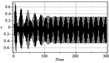
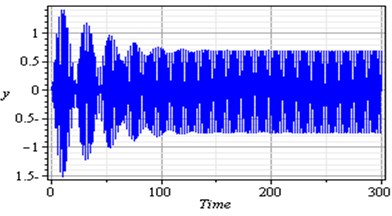
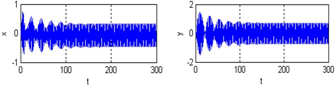
The differential equation of the rotor-seal system is solved numerically using Rung-Kutta fourth order method and MATLAB, MAPLE packages as shown in Figs. 2-4. Fig. 2 illustrates the response and the phase-plane for the non-resonant rotor-seal system (basic case) where $Ω \neq ω_{1} \neq ω_{2}$ at some practical values of the equation parameters $α_{1} = 0.03,$ $α_{2} = 0.0001,$ $α_{3} =$ –0.05, $α_{4} =$ –0.2, $α_{5} = 0.01$ , $α_{6} = 0.02$ , $α_{7} = 0.25$ , $α_{8} = 0.004$ , $α_{9} = 0.7$ , $α_{10} =$ –0.8, $α_{11} =$ –0.2, $α_{12} = 0.004$ , $α_{13} = 0.01$ , $α_{14} = 0.02$ , $α_{15} = 0.003$ , $α_{16} =$ –0.04, $α_{17} = 0.001,$ $α_{18} =$ –0.5, $α_{19} =$ –0.03, $α_{20} =$ –0.04, $α_{21} = 0.5$ , $β_{1} = 0.05$ , $β_{2} = 0.2$ , $β_{3} =$ –0.03, $β_{4} = 0.0001$ , $β_{5} = 0.002$ , $β_{6} = 0.01$ , $β_{7} = 0.2$ , $β_{8} = 0.004$ , $β_{9} = 0.8$ , $β_{10} = 0.7$ , $β_{11} =$ –0.25, $β_{12} =$ –0.01, $β_{13} =$ –0.004, $β_{14} = 0.03$ , $β_{15} =$ –0.001, $β_{16} = 0.5$ , $β_{17} =$ –0.003, $β_{18} = 0.04$ , $β_{19} =$ –0.02, $β_{20} =$ –0.5, $β_{21} = 0.04$ , $Ω = 3$ , $ω_{1} = 2.8$ , $ω_{2} = 3.25$ , $ρ = 1$ . It is observed from this Fig. 2 that the response of the first and second modes of the rotor-seal system start with increasing amplitude and becomes stable respectively and the steady state amplitudes $x$ and $y$ are about 0.3 and 0.7 respectively and the phase plane shows limit cycle, denoting that the system is free from chaos. Table 1 shows the results of the worst resonance conditions.

Fig. 2Non-resonance rotor-seal system response (basic case)

For the simultaneous primary and internal resonance ( $Ω ≅ ω_{1}$ and $ω_{2} ≅ 3 ω_{1}$ ) which is one of the worst resonance cases as shown in Fig. 3, it can be shown that for the first and second modes of the rotor-seal system, the steady state amplitudes are increased to about 670 % and 1140 % respectively of that values shown in Fig. 2. The vibration of the first mode is increased and become stable with tuned oscillation. Also the response of the second mode is increased and becomes stale with some chaotic. The phase-plane shows a multi-limit cycle for the first and second modes.

Fig. 4 shows that the time response and phase-plane of the simultaneous primary and internal resonance ( $Ω ≅ ω_{1}$ and $ω_{2} ≅ ω_{1}$ ) which another one of the worst resonance cases. From this figure we have that the amplitude of the first mode of the rotor-seal system is increased to about 670 % while the amplitude of the second mode is increased to about 570 % of the of that values shown in Fig. 2. The oscillations of the first and second modes become stable, chaotic and tuned and the phase plane shows multi-limit cycle.

5.1. Effects of different parameters

In this section, the effects of different parameters near the simultaneous primary and internal resonance case is investigated and studied. The frequency response equations are given by Eqs. (37) and (38) are solved numerically at the same values of the parameters shown in Fig. 2. In all figures, the solid lines stand for the stable solution and the dashed lines for the unstable solution.

Table 1Summary of the worst resonance cases

Resonance cases	$x$ (%)	$y$ (%)	Remarks
Non-resonance case	100 %	100 %	Limit cycle
$Ω ≅ ω_{1}$	700 %	620 %	Multi limit cycle
$Ω ≅ \frac{ω_{1}}{2}$	560 %	570 %	Multi limit cycle
$Ω ≅ \frac{ω_{1}}{3}$	560 %	580 %	Multi limit cycle
$Ω ≅ \frac{2 ω_{1}}{3}$	600 %	570 %	Multi limit cycle
$Ω ≅ \frac{3 ω_{1}}{2}$	500 %	530 %	Multi limit cycle
$Ω ≅ \frac{ω_{2}}{2}$	560 %	570 %	Multi limit cycle
$Ω ≅ \frac{ω_{2}}{3}$	560 %	580 %	Multi limit cycle
$Ω ≅ \frac{2 ω_{2}}{3}$	600 %	570 %	Multi limit cycle
$Ω ≅ \frac{3 ω_{2}}{2}$	500 %	500 %	Multi limit cycle
$Ω ≅ ω_{1}, ω_{2} ≅ ω_{1}$	670 %	570 %	Multi limit cycle
$Ω ≅ ω_{1}, ω_{2} ≅ 2 ω_{1}$	730 %	1000 %	Multi limit cycle
$Ω ≅ ω_{1}, ω_{2} ≅ 3 ω_{1}$	670 %	1140 %	Multi limit cycle
$Ω ≅ ω_{1}, ω_{2} ≅ 4 ω_{1}$	370 %	200 %	Multi limit cycle
$Ω ≅ ω_{1}, ω_{2} ≅ 5 ω_{1}$	800 %	240 %	Multi limit cycle
$Ω ≅ ω_{1}, ω_{2} ≅ \frac{ω_{1}}{2}$	85 %	320 %	Multi limit cycle
$Ω ≅ ω_{1}, ω_{2} ≅ \frac{ω_{1}}{3}$	400 %	530 %	Multi limit cycle
$Ω ≅ ω_{1}, ω_{2} ≅ \frac{ω_{1}}{4}$	200 %	430 %	Multi limit cycle
$Ω ≅ ω_{1}, ω_{2} ≅ \frac{2 ω_{1}}{3}$	220 %	320 %	Multi limit cycle
$Ω ≅ ω_{2}, ω_{1} ≅ ω_{2}$	830 %	430 %	Multi limit cycle
$Ω ≅ ω_{2}, ω_{1} ≅ 2 ω_{2}$	85 %	430 %	Multi limit cycle
$Ω ≅ ω_{2}, ω_{1} ≅ 3 ω_{2}$	50 %	500 %	Multi limit cycle
$Ω ≅ ω_{2}, ω_{1} ≅ 4 ω_{2}$	35 %	570 %	Multi limit cycle
$Ω ≅ ω_{2}, ω_{1} ≅ 5 ω_{2}$	20 %	570 %	Multi limit cycle
$Ω ≅ ω_{2}, ω_{1} ≅ \frac{ω_{2}}{2}$	720 %	930 %	Multi limit cycle
$Ω ≅ ω_{2}, ω_{1} ≅ \frac{2 ω_{2}}{3}$	670 %	860 %	Multi limit cycle
$Ω ≅ ω_{2}, ω_{1} ≅ \frac{3 ω_{2}}{2}$	100 %	530 %	Multi limit cycle
$Ω ≅ 2 ω_{1}, ω_{2} ≅ ω_{1}$	670 %	290 %	Multi limit cycle
$Ω ≅ 2 ω_{1}, ω_{2} ≅ 4 ω_{1}$	530 %	170 %	Multi limit cycle
$Ω ≅ 3 ω_{1}, ω_{2} ≅ ω_{1}$	430 %	290 %	Multi limit cycle
$Ω ≅ 3 ω_{1}, ω_{2} ≅ 3 ω_{1}$	730 %	1190 %	Multi limit cycle

Fig. 3Simultaneous primary and internal resonance case (Ω≅ω1 and ω2≅3ω1)

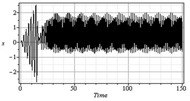
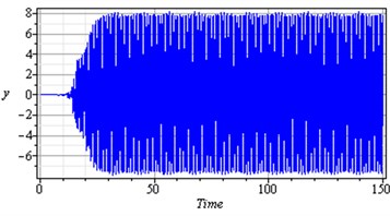
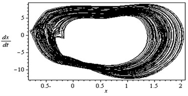
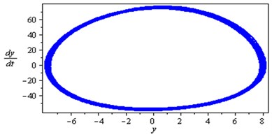
Fig. 4Simultaneous primary combined and internal resonance case (Ω≅ω1 and ω2≅ω1)

5.1.1. Response curves of the first mode

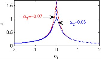
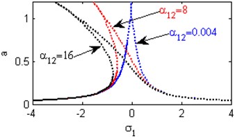
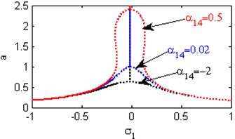
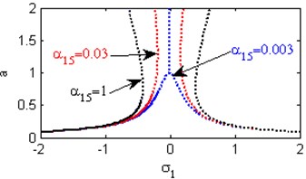
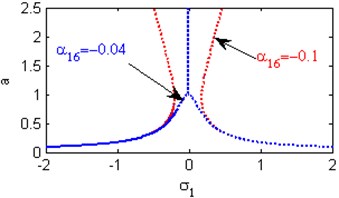
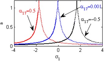
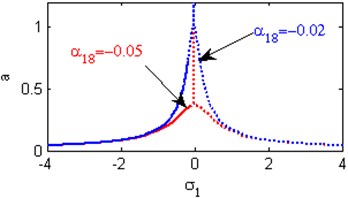
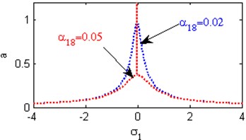
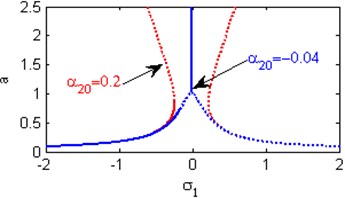
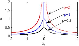
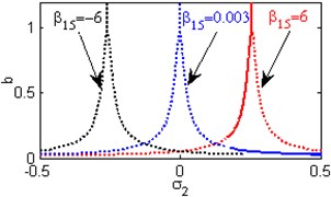
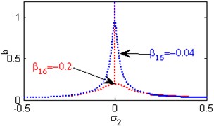
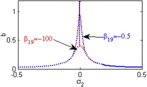
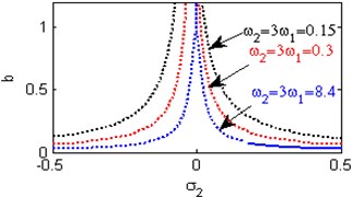
Fig. 5(a) shows the steady state amplitudes of the first mode against the detuning parameter $σ_{1}$ at the practical case, where $a \neq 0$ , $b \neq 0$ . For increasing values of the nonlinear parameter $α_{1}$ and $α_{17}$ , the curves are shifted to the left and the regions of stability are increased as shown in Figs. 5(b) and 5(j). Fig. 5(c) shows that the steady state amplitude of the first mode is a monotonic decreasing function in the linear damping coefficients $α_{2}$ . Fig. 5(d) shows that the steady state amplitude of the first mode is a monotonic increasing function in the nonlinear parameter $α_{12}$ and the response curves are bent to the left leading to the occurrence of the jump phenomena, multi-valued amplitudes and the regions of stability are decreased. The steady state amplitude of the first mode is a monotonic increasing function in the nonlinear parameter $α_{14}$ and the excitation amplitudes $ρ$ and the regions of instability are increased as shown in Figs. 5 (e) and 5(o). For increasing values of the nonlinear parameter $α_{15}$ , $α_{16}$ and $α_{20}$ the steady state amplitude of the first mode is increased and the curves are diverged as shown in Figs. 5(f), 5(h), 5(m). For negative values of the nonlinear parameter $α_{15}$ and $α_{18}$ , the steady state amplitude of the first mode is increased and the stability regions are increased as shown in Figs. 5(g) and 5(k). Figs. 5(i), 5(l) show that, for positive values of the nonlinear parameter $α_{16}$ and $α_{18}$ , the system is unstable. Fig. 5(n) shows that the steady state amplitude of the first mode is a monotonic decreasing function in the natural frequencies $ω_{1}$ and $ω_{2}$ .

Fig. 5Effects of different parameters on the first mode

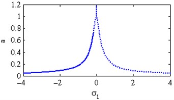
a) Effects of the detuning parameter $σ_{1}$

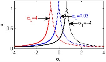
b) Effects of the non-linear parameter $α_{1}$

c) Effects of the damping coefficient $α_{2}$

d) Effects of the non-linear parameter $α_{12}$

e) Effects of the non-linear parameter $α_{14}$

f) Effects of the non-linear parameter $α_{15}$

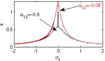
g) Effects of the non-linear parameter $α_{15}$

h) Effects of the non-linear parameter $α_{16}$

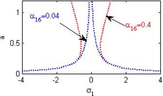
i) Effects of the non-linear parameter $α_{16}$

j) Effects of the non-linear parameter $α_{17}$

k) Effects of the non-linear parameter $α_{18}$

l) Effects of the non-linear parameter $α_{18}$

m) Effects of the non-linear parameter $α_{20}$

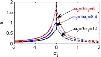
n) Effects of the natural frequencies $ω_{1}$ , $ω_{2}$

o) Effects of the excitation amplitude $ρ$

5.1.2. Response curves of the second mode

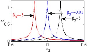
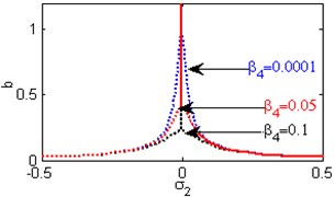
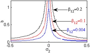
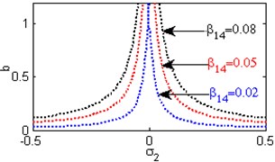
Fig. 6(a) shows the steady state amplitudes of the second mode against the detuning parameter $σ_{2}$ at the practical case, where $a \neq 0$ , $b \neq 0$ . For increasing values of the nonlinear parameter $β_{3}$ and $β_{15}$ , the curves are shifted to the right leading to the occurrence of the jump phenomena, multi-valued amplitudes as shown in Figs. 6(b) and 6(h). Figs. 6(c), 6(f), 6(k) show that the steady state amplitudes of the second mode are monotonic decreasing functions in the linear damping coefficients $β_{4}$ , the nonlinear parameter $β_{14}$ and the natural frequencies $ω_{1}$ and $ω_{2}$ . Figs. 6(d), 6(i), 6(j) shows that the steady state amplitudes of the second mode are monotonic increasing functions in the nonlinear parameters $β_{12}$ , $β_{16}$ and $β_{19}$ . For negative and positive values of the nonlinear parameter $β_{13}$ , the steady state amplitude of the second mode is trivial leading to the occurrence of the saturation phenomena as shown in Fig. 6(e). For increasing positive values of the nonlinear parameter $β_{14}$ , the steady state amplitude of the second mode is increased and the system is unstable as shown in Fig. 6(g). The regions of stability are decreased for increasing values of the nonlinear parameters $β_{3}$ and $β_{12}$ . The regions of stability are increased for increasing values of the nonlinear parameter $β_{15}$ and the natural frequencies $ω_{1}$ and $ω_{2}$ .

Fig. 6Effects of different parameters on the second mode

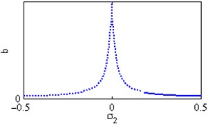
a) Effects of the detuning parameter $σ_{2}$

b) Effects of the non-linear parameter $β_{3}$

c) Effects of the damping coefficient $β_{4}$

d) Effects of the non-linear parameter $β_{12}$

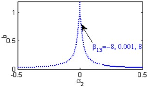
e) Effects of the non-linear parameter $β_{13}$

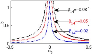
f) Effects of the non-linear parameter $β_{14}$

g) Effects of the non-linear parameter $β_{14}$

h) Effects of the non-linear parameter $β_{15}$

i) Effects of the non-linear parameter $β_{16}$

j) Effects of the non-linear parameter $β_{19}$

k) Effects of the natural frequencies $ω_{1}$ , $ω_{2}$

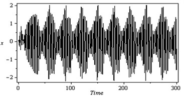
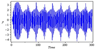
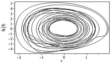
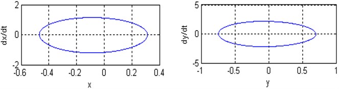
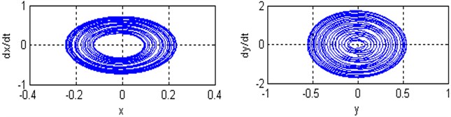
Fig. 7a), b) Time responses and phase plane of the coupled system respectively; c) Poincare maps of the coupled system respectively; for (Ω=3, ω1=2.8, ω2=3.25 and ρ=1)

a), b) Time responses and phase plane of the coupled system respectively; c) Poincare maps of the coupled system respectively; for (Ω=3, ω1=2.8, ω2=3.25 and ρ=1)

a)

b)

c)

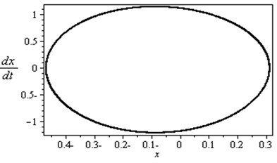
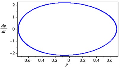
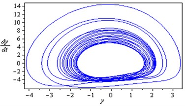
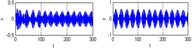
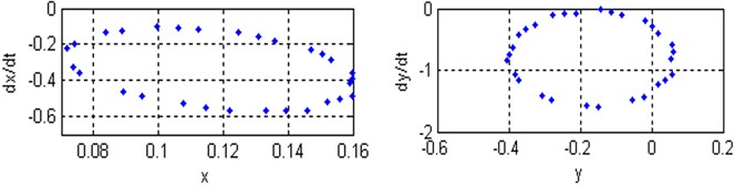
Fig. 8a), b) Time responses and phase plane of the coupled system respectively; c) Poincare maps of the coupled system respectively; for (Ω=3, ω1=2.8, ω2=3.25 and ρ=0.4)

a), b) Time responses and phase plane of the coupled system respectively; c) Poincare maps of the coupled system respectively; for (Ω=3, ω1=2.8, ω2=3.25 and ρ=0.4)

a)

b)

c)

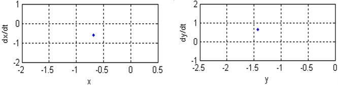
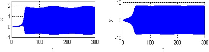
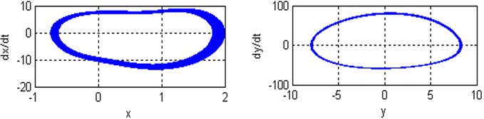
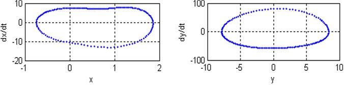
Fig. 9a), b) Time responses and phase plane of the coupled system respectively; c) Poincare maps of the coupled system respectively; for (Ω=8.4, ω1=2.8, ω2=8.4 and ρ=1)

a), b) Time responses and phase plane of the coupled system respectively; c) Poincare maps of the coupled system respectively; for (Ω=8.4, ω1=2.8, ω2=8.4 and ρ=1)

a)

b)

c)

6. Poincare map

Poincare maps are introduced via example using two-dimensional autonomous systems of differential equations. They are used extensively to transform complicated behavior in the phase space to discrete maps in a lower-dimensional space. Poincaré maps are used to determine stability and plot bifurcation diagrams. By simulating the movement of rotor-seal system (2) and Poincare mapping, the Fig. 7-9 are obtained. At $ρ = 1$ with the non-resonant rotor-seal system where $Ω \neq ω_{1} \neq ω_{2}$ , there is a period-one harmonic solution, which is depicted as a closed curve in the phase plane and as and there exist one isolated points on Poincare map as shown in Fig. 7. When $ρ = 0.4$ with the non-resonant rotor-seal system where $Ω \neq ω_{1} \neq ω_{2}$ , the system becomes chaotic and quasi-periodic motion appears and a close curve is observed on Poincare map as shown in Fig. 8. Fig. 9 shows that the time response of the rotor-seal system become stable and quasi-periodic motion appears at $ρ = 1$ with the simultaneous sub-harmonic and internal resonance case ( $Ω ≅ 3 ω_{1}$ , $ω_{2} ≅ 3 ω_{1}$ ).

7. Conclusions

Multiple time scale perturbation method is useful to determine approximate solutions for the coupled nonlinear differential equations describing the rotor-seal system up to and including the second order approximation. It is quite clear that some of the simultaneous resonance cases are undesirable in the design of such system as they represent some of the worst behavior of the system. Both the frequency response equations and the phase-plane technique are applied to study the stability of the system. The effect of the different parameters of the system is studied numerically. From the above study the following may be concluded:

1) The amplitude of the first mode is increased to about 30 % of the maximum excitation forces amplitude $ρ$ , while the amplitude of the second mode is increased to about 70 % at the non-resonant case ( $Ω \neq ω_{1} \neq ω_{2}$ ).

2) The amplitude of the first mode is increased to about 670 % while the amplitude of the second mode is increased to about 1140 % at resonance case ( $Ω ≅ ω_{1}$ and $ω_{2} ≅ 3 ω_{1}$ ).

3) The amplitude of the first mode is increased to about 670 % while the amplitude of the second mode is increased to about 570 % at resonance case ( $Ω ≅ ω_{1}$ and $ω_{2} ≅ ω_{1}$ ).

4) The regions of stability are increased for increasing values of $α_{1}$ , $α_{14}$ and $α_{17}$ .

5) For positive values of the nonlinear parameter $α_{16}$ and $α_{18}$ , the system become unstable.

6) For increasing values of the nonlinear parameter $β_{3}$ and $β_{15}$ , the curves are shifted to the right leading to the occurrence of the jump phenomena, multi-valued.

7) For negative and positive values of the nonlinear parameter $β_{13}$ , the steady state amplitude of the second mode is trivial leading to the occurrence of the saturation phenomena.

References

Dimarogonas A. D., Gomez-Mancilla J. C. Flow-excited turbine rotor instability. International Journal of Rotating Machinery, Vol. 1, Issue 1, 1994, p. 3-51.

Search CrossRef
Marquette O. R., Childs D. W., Andres L. S. Eccentricity effects on the rotor dynamic coefficients of plain annular seals theory versus experiment. ASME Journal of Tribology, Vol. 119, Issue 3, 1997, p. 443-447.

Search CrossRef
Klaus K. Dynamic coefficients of stepped labyrinth gas seals. Journal of Engineering for Gas Turbines and Power, Vol. 122, Issue 3, 2000, p. 473-477.

Search CrossRef
Dietzed F. J., Nordmann R. Calculating coefficients of seals by finite-difference techniques. SME Journal of Tribology, Vol. 109, Issue 3, 1987, p. 388-394.

Search CrossRef
Toshio H., Guo Z. L., Gordon K. R. Application of fluid dynamics analysis for rotating machinery – part II: labyrinth seal analysis. Journal of Engineering for Gas Turbines and Power, Vol. 127, Issue 4, 2005, p. 820-826.

Search CrossRef
Alford J. S. Protecting turbomachinery from self-excited rotor whirl. ASME Journal of Engineering for Power, Vol. 87, Issue 4, 1965, p. 333-344.

Search CrossRef
Ding Q., Zhang K. Order reduction and nonlinear behaviors of a continuous rotor system. Nonlinear Dynamics, Vol. 67, 2012, p. 251-262.

Search CrossRef
Chen Y. M., Meng G., Liu J. K. A new method for Fourier series expansions: applications in rotor-seal systems. Mechanics Research Communications, Vol. 38, 2011, p. 399-403.

Search CrossRef
Li W., Yang Y., Sheng D., Chen J. A novel nonlinear model of rotor/bearing/seal system and numerical analysis. Mechanism and Machine Theory, Vol. 46, 2011, p. 618-631.

Search CrossRef
Zhang H., Chen Y. Bifurcation analysis on full annular rub of a nonlinear rotor system. Science China, Technological Sciences, Vol. 54, Issue 8, 2011, p. 1977-1985.

Search CrossRef
Cheng M., Meng G., Jing J. Non-linear dynamics of a rotor-bearing-seal system. Archive of Applied Mechanics, Vol. 76, 2006, p. 215-227.

Search CrossRef
Ding Q., Cooper J. E., Leung A. Y. T. Hopf bifurcation analysis of a rotor-seal system. Journal of Sound and Vibration, Vol. 252, Issue 5, 2002, p. 817-833.

Search CrossRef
Li Z., Chen Y. Research on 1:2 subharmonic resonance and bifurcation of nonlinear rotor-seal system. Applied Mathematics and Mechanics, Vol. 33, Issue 4, 2012, p. 499-510.

Search CrossRef
Sayed M., Mousa A. A. Second-order approximation of angle-ply composite laminated thin plate under combined excitations. Communication in Nonlinear Science and Numerical Simulation, Vol. 17, 2012, p. 5201-5216.

Search CrossRef
Eissa M., Sayed M. A comparison between passive and active control of non-linear simple pendulum, part-I. Mathematical and Computational Applications, Vol. 11, 2006, p. 137-149.

Search CrossRef
Eissa M., Sayed M. A comparison between passive and active control of non-linear simple pendulum, part-II. Mathematical and Computational Applications, Vol. 11, 2006, p. 151-162.

Search CrossRef
Eissa M., Sayed M. Vibration reduction of a three DOF non-linear spring pendulum. Communication in Nonlinear Science and Numerical Simulation, Vol. 13, 2008, p. 465-488.

Search CrossRef
Sayed M. Improving the mathematical solutions of nonlinear differential equations using different control methods. Ph. D. Thesis, Menofia University, Egypt, 2006.

Search CrossRef
Amer Y. A., Bauomy H. S., Sayed M. Vibration suppression in a twin-tail system to parametric and external excitations. Computers and Mathematics with Applications, Vol. 58, 2009, p. 1947-1964.

Search CrossRef
Sayed M., Hamed Y. S. Stability and response of a nonlinear coupled pitch-roll ship model under parametric and harmonic excitations. Nonlinear Dynamics, Vol. 64, 2011, p. 207-220.

Search CrossRef
Hamed Y. S., El-Ganaini W. A., Kamel M. M. Vibration suppression in ultrasonic machining described by non-linear differential equations. Journal of Mechanical Science and Technology, Vol. 23, Issue 8, 2009, p. 2038-2050.

Search CrossRef
Hamed Y. S., El-Ganaini W. A., Kamel M. M. Vibration suppression in multi-tool ultrasonic machining to multi-external and parametric excitations. Acta Mechanica Sinica, Vol. 25, 2009, p. 403-415.

Search CrossRef
Hamed Y. S., El-Ganaini W. A., Kamel M. M. Vibration reduction in ultrasonic machine to external and tuned excitation forces. Applied Mathematical Modeling, Vol. 33, 2009, p. 2853-2863.

Search CrossRef
Hamed Y. S., Sayed M., Cao D.-X., Zhang W. Nonlinear study of the dynamic behavior of a string-beam coupled system under combined excitations. Acta Mechanica Sinica, Vol. 27, Issue 6, 2011, p. 1034-1051.

Search CrossRef
Sayed M., Kamel M. Stability study and control of helicopter blade flapping vibrations. Applied Mathematical Modelling, Vol. 35, 2011, p. 2820-2837.

Search CrossRef
Sayed M., Kamel M. 1:2 and 1:3 internal resonance active absorber for non-linear vibrating system. Applied Mathematical Modelling, Vol. 36, 2012, p. 310-332.

Search CrossRef
Sayed M., Hamed Y. S., Amer Y. A. Vibration reduction and stability of non-linear system subjected to external and parametric excitation forces under a non-linear absorber. International Journal of Contemporary Mathematical Sciences, Vol. 6, Issue 22, 2011, p. 1051-1070.

Search CrossRef
Sayed M., Mousa A. A. Vibration, stability, and resonance of angle-ply composite laminated rectangular thin plate under multi-excitations. Mathematical Problems in Engineering, 2013.

Search CrossRef
Poincaré H. Memory on the curves defined by a differential equation. Journal de Mathématiques Pures et Appliquées, Vol. 7, 1881, p. 375-422.

Search CrossRef
Nayfeh A. H. Introduction to Perturbation Techniques. John Wiley & Sons, Inc., New York, 1981.

Search CrossRef
Nayfeh A. H. Non-linear Interactions. Wiley-Inter-Science, New York, 2000.

Search CrossRef

About this article

Received

13 January 2014

Accepted

02 December 2014

Published

30 December 2014

Keywords

multiple time scale

resonance cases

stability

Acknowledgements

The authors would like to express their gratitude to the Editor and Referees for their encouragement and constructive comments in revising the paper.

This is an open access article distributed under the Creative Commons Attribution License, which permits unrestricted use, distribution, and reproduction in any medium, provided the original work is properly cited.