Abstract
The system of suspended cable with mixed excitation forces is controlled in this paper by using negative linear velocity feedback controller. The equations of motion of this system contain quadratic and cubic nonlinearities. The multiple scale perturbation technique is applied to determine the response of the nonlinear system near the simultaneous sub-harmonic and combined resonance case of this system. The stability of the obtained numerical solution is investigated using frequency response equations. The effect of different parameters on the vibrating system are investigated and reported.
1. Introduction
Suspended cables are lightweight, flexible structural elements used in numerous applications in mechanical, civil, electrical, ocean, and space engineering due to their capability of transmitting forces, carrying payloads, and conducting signals across large distances. At the same time, the suspended cable is a basic element of theoretical interest in applied mechanics and an archetypal model of various phenomena in dynamics. Arafat and Nayfeh [1] studied the motion of shallow suspended cables with primary resonance excitation. The method of multiple scales is applied to study nonlinear response of this suspended cables, its stability and the dynamic solutions. Some interesting work on the nonlinear dynamics of cables to harmonic excitations can be found in the review articles by Rega [2, 3]. Zheng et al. [4] considered the super-harmonics and internal resonance of a suspended cable with almost commensurable natural frequencies. Zhang and Tang [5] investigated the chaotic dynamics and global bifurcations of the suspended inclined cable under combined parametric and external excitations. Chen and Xu [6] investigated the global bifurcations of the inclined cable subjected to a harmonic excitation leading to primary resonances with the external damping by using averaging method. Benedettini et al. [7] studied nonlinear oscillations of a four-degree-of-freedom model of the sus- pended cables under multiple internal resonance conditions. They have established that the response of suspended cables near or away from the first crossover can be large and exhibit very complex behavior due to the simultaneous presence of multiple internal resonances involving several in-plane modes and out-of-plane modes.
Kamel and Hamed [8] analyzed the nonlinear behavior of an elastic cable subjected to harmonic excitation near the simultaneous principle primary and internal resonance using multiple scale method. The numerical solutions and chaotic response of the nonlinear system of elastic cable for different parameters are also studied. Abe [9] investigated the accuracy of nonlinear vibration analyses of a suspended cable, which possesses quadratic and cubic nonlinearities, with 1:1 internal resonance. The nonlinear dynamics of suspended cable structures have been studied with 2:1 internal resonances by the authors [10, 11]. Chen et al. [12] studied the bifurcations and chaotic dynamics of the parametrically and externally excited suspended elastic cable. A sample suspended cable, representing a physical model is considered as the case study, and non-collocated feedback, based on active transverse control, is considered as a final application of the state observer. Also, active feedback control for cable vibrations is studied by Ubertini [13] for analytical and numerical models. A suitable dimensional analytical Galerkin model is derived to investigate the effectiveness of the feedback control, which represents the final application of the state observer.
Wang and Zhao [14-16] applied different methods to investigate the nonlinear response of the suspended cable with three-to-one internal resonance, and numerical simulations are used to illustrate the chaotic dynamics of the cable. They also extended the previous work to consider the out-of-plane motion of a shallow suspended cable [17]. The three-to-one internal resonance between the third and the first symmetric in-plane modes and the one-to-one internal resonance between the third symmetric in-plane mode and the third symmetric out-of-plane mode are taken in to account. The case of the primary resonance of the first symmetric mode is also considered. Sofi and Muscolino [18] studied the dynamics of suspended cables with small sag-to-span ratios carrying an array of moving oscillators with arbitrarily varying velocities. Numerical results demonstrate that, despite the basis functions are continuous; the improved series enables to capture with very few terms the abrupt changes of cable profile at the contact points between the cable and the moving oscillators. Wang and Rega [19] obtained the 3D nonlinear equations of motion of the suspended cable with moving mass via the Hamilton principle, and its transient linear planar dynamics is investigated. They studied the transient response of the suspended cable subjected to a sequence of masses moving with constant velocity. The numerical results show that the effect of the velocity on the maximum mid span displacement is very small. Huang et al. [20] obtained the nonlinear ordinary differential equations (ODEs) by the Galerkin method from the nonlinear partial differential equations (PDEs) to describe the forced vibration of the coupled structure of a suspended-cable-stayed beam. The multiple-scale method is employed to solve the ODEs. They found that there are typical jumps and saturation phenomena of the vibration amplitude in the structure and the structure may present quasi-periodic vibration or chaos, if the stiffness of the cable stays membrane and frequency of external excitation are disturbed. The control strategies proposed in the literature often involve the application of control command to various parts of the crane, such as the cables [21-23]. Hamed and Amer [24] studied an active vibration controller for suppressing the vibration of the non-linear composite beam subjected to parametric excitation force in the presence of 1:2 internal resonances. The numerical results show that the saturation control of steady state vibrations is efficient. Al-Qassab et al. [25] investigated the dynamic behavior of an elastic horizontal and inclined cable with a moving mass along its length. Kim and Chang [26] analyzed the free vibration and presented a dynamic stiffness matrix for an inclined cable. F. Xu et al. [27] introduced an analyzing method and initial experimental method to study coupling dynamic characteristics of cable-robot system. The experimental results validate the theoretical vibration characteristics, including frequency, vibration amplitude, and acceleration.
The aim of this work is to control a two degree of freedom nonlinear differential equations of a suspended cable having quadratic and cubic nonlinearities subjected to mixed excitations via a negative velocity feedback controller. The method of multiple scales perturbation [28] is applied to solve the nonlinear differential equations describing the controlled system up to second order approximations. The behavior of the system is studied applying Runge-Kutta fourth-order method. The stability of the proposed analytic nonlinear solution near the simultaneous sub-harmonic and combined resonance case is studied numerically. The stability of the system is investigated applying frequency response equations. The effect of different parameters on the steady state responses of the vibrating system is studied and discussed from the frequency response curves.
2. Mathematical reduction from PDEs to ODEs
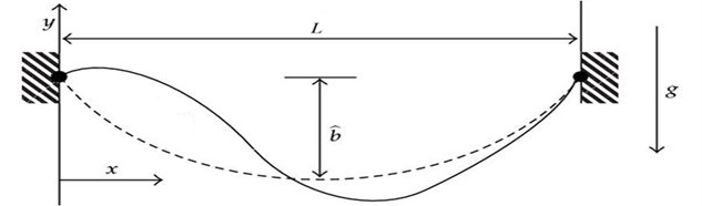
Following Benedettini et al. [7], we express the dimensional non-planar equations of motion for a shallow suspended elastic cable hanging at fixed supports and caused by axial excitation and horizontal load as shown in Fig. 1, is as follows:
where, for a sag-to-span ratio , the static equilibrium profile of the cable may be sufficiently approximated by a parabola. Hence:
wheere, and denote the in-plane (in-plane; i.e., the plane defined by the initial static configuration of the cable) and out-of-plane displacements at position at time , is the mass per unit length, is the cable sag, is the cable span, is Young’s modulus, is the area of the cross section, are viscous damping coefficients, and is the gravitational acceleration.
Fig. 1A schematic diagram of a shallow suspended cable
The boundary conditions are:
We introduce non-dimensional quantities defined by:
into Eqs. (1) and (2), where the characteristic time will be chosen at the end of the analysis, and obtain the following non-dimensional non-planar equations of motion:
where and the boundary conditions are:
The overdot and prime indicate the derivatives with respect to and, respectively, and:
In order to analyze the nonlinear responses of this system, we first discretize Eq. (5) using the Galerkin procedure. To this end, we express the in-plane and out-of-plane displacements and as:
where the and are the modes shapes of the linearized problem, and are generalized coordinates. Substituting Eq. (8) into Eq. (5), the two-degree-of-freedom nonlinear equations can be obtained as follows:
where and refer to the vertical (in-plane) and horizontal (out-of-plane) displacements, respectively, and are viscous damping coefficients, is a small parameter, and respectively, represent the natural frequencies associated with the anti-symmetric or symmetric in-plane and out-of-plane modes, , , , ( 2, 3) are nonlinear coefficients, , are the excitation frequencies, , are the parametric excitation force amplitudes of the cable and is the external excitation force amplitude of the cable.
3. Perturbation analysis
Our attention is focused on a suspended cable excited by harmonic, parametric and tuned excitation forces. The two-degree-of- freedom differential equations describing the nonlinear dynamics of the suspended cable [12] can be investigated as:
where and are the control forces which added to the system, , are the excitation frequencies, is the tuned excitation force amplitude of the cable and , are the positive constants (gains).
Assuming the solution of Eqs. (11) and (12) in the forms:
where, , (0, 1), and are the fast and slow time scales respectively.
The derivatives will be in the form:
where , 0, 1.
Substituting from Eqs. (13) and (14) into Eqs. (11) and (12) and equating the same power of we have:
The general solutions of Eqs. (17) and (18) can be written in the form:
where , are complex functions in and denotes the complex conjugate functions. Substituting Eqs. (21) and (22) into Eqs. (19) and (20), we get:
Eliminating the secular terms of Eqs. (23) and (24) to get bounded solutions, then the general solution of the resulting equations obtained as:
From the Eqs. (25) and (26), the deduced resonance cases are:
(i) Primary resonance: , ;
(ii) Sub-harmonic resonance: , ;
(iii) Internal resonance: , 1, 2;
(iv) Combined resonance: , ;
(iiv) Simultaneous resonance: Any combination of the above resonance cases is considered as simultaneous resonance.
4. Stability analysis
The stability of the considered system is investigated at the worst resonance case (confirmed numerically), which is the simultaneous sub-harmonic and combined resonance case, where Consider the resonance conditions and , where and are called the detuning parameters and eliminating the secular terms from the first approximations of Eqs. (23) and (24) leads to solvability conditions as:
Using the polar form:
where , and , are the steady state amplitudes and phases of the motions respectively. Substituting from Eq. (29) into Eqs. (27) and (28) and equating imaginary and real parts, we obtain:
where, and are phases of motion.
For steady-state solutions, we put , 1, 2 to Eqs. (30)-(33) we get the following:
From Eqs. (34)-(37) we have the following cases:
(i) 0, , (ii) 0, 0 and (iii) 0, 0 (practical case).
For the practical case (0, 0), Squaring Eqs. (34) and (35), then adding the squared results together, similarly to Eqs. (36) and (37) gives the following frequency response equations:
On the way to determine the stability of the fixed point solutions of Eqs. (34)-(37), we introduce the following forms:
where , , , are real coefficients. Substitution from Eq. (40) into the linear form of Eqs. (27) and (28), that is:
Substituting from Eq. (40) into Eqs. (41) and (42) and equating the imaginary and real parts of Eq. (41) and Eq. (42) we contain:
The stability of a particular fixed point with respect to a proportional to (where is an eigenvalue) is determined by zeros of the characteristic equation:
To analyze the stability of the non-trivial solution, one uses Eq. (47) to obtain:
where:
are constants. According to the Routh-Hurwitz criterion, the necessary and sufficient conditions for all the roots of Eq. (48) to possess negative real parts are: 0, 0, and .
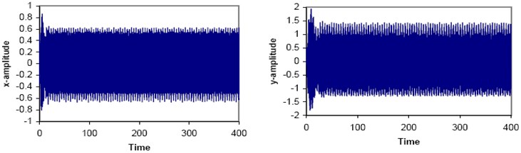
Fig. 2Non-resonant time response solution at selected values: cx= 0.2, α2= 0.3, β2= 0.2, γ2=0.3, η2= 0.4, cy= 0.1, α3= 0.1, γ3= 0.1, η3= 0.1, ωx= 7.5, ωy= 7.8, Ω= 1.4, Ω1= 5.3, Ω2= 4.75, Ω3= 3.35, f1= 4.0, f2= 3.0, F= 2.0, Q= 4.0
5. Numerical results
5.1. Active control effect
In order to verify the analytic results, the equations of motion Eqs. (11) and (12) is numerically integrated using a fourth order Runge-Kutta algorithm. Fig. 2 shows the non-resonant system behavior, where the maximum steady state amplitudes and are about 30 % and 70 % of the external excitation amplitude respectively, this case can be regarded as a basic case. The worst resonance case of the system is the simultaneous sub-harmonic and combined resonance case , , where the steady-state amplitudes are increased to about 250 % and 200 %. We added a negative linear velocity feedback to this worst resonance case as shown in Fig. 3. We found that the vibration amplitudes of the system are decreased. Best effectiveness of the system is obtained when the linear velocity feedback controller added to the system. The effectiveness of the controller is determined from the relation ( steady state amplitude of the system without controller/steady state amplitude of the system with controller), where ( 2000 % for the amplitude and 800 % for the amplitude ) at the worst resonance case which is the simultaneous sub- harmonic and combined resonance case.
Fig. 3Simultaneous sub-harmonic and combined resonance case (Ω1≅2ωx, Ω2+Ω3≅ωy)
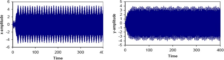
a) System without controller
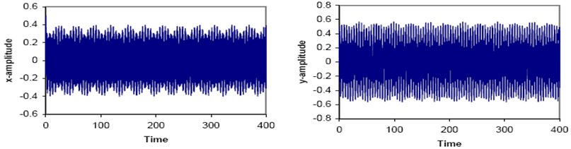
b) System with negative linear velocity feedback controller (2.0)
Table 1Numerical solutions of frequency response equations
Parameters | Effect | Fig. 4(a) () | Parameters | Effect | Fig. 5(a) () |
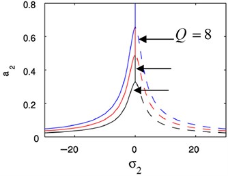
Excitation force | M.I. | Fig. 4(b) | Excitation force | M.I. | Fig. 5(b) |
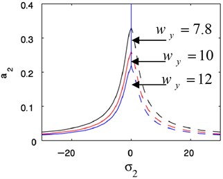
Natural frequency | M.I. with R.D. | Fig. 4(c) | Natural frequency | M.D. | Fig. 5(c) |
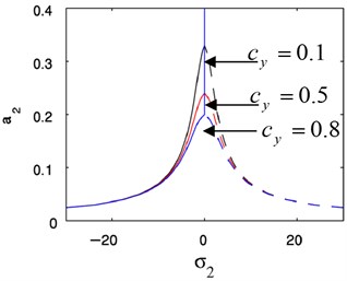
Damping coefficient | M.D. | Fig. 4(d) | Damping coefficient | M.D. | Fig. 5(d) |
Non-Linear parameter | H&S | Fig. 4(e) | Non-Linear parameter | H&S | Fig. 5(e) |
Non-Linear parameter | S.A. | Fig. 4(f) | Non-Linear parameter | SA. | Fig. 5(f) |
Gain | M.D. | Fig. 4(g) | Gain | M.D. | Fig. 5(g) |
M.I. | Fig. 4(h) | M.I. | Fig. 5(h) | ||
M.I. denotes that the amplitude is monotonic increasing function in the parameter; M.D. denotes that the amplitude is monotonic decreasing function in the parameter; R.D. denotes that the region is decreased; S.A. denotes that the amplitude is Saturation; H&S means that the parameter has hardening and softening non-linearity effects. | |||||
5.2. Response curves and effects of different parameters
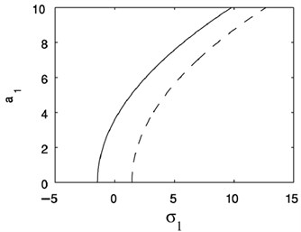
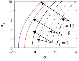
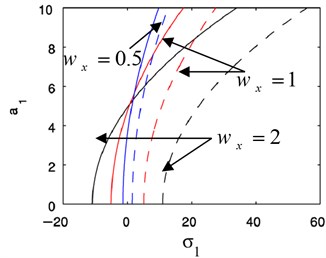
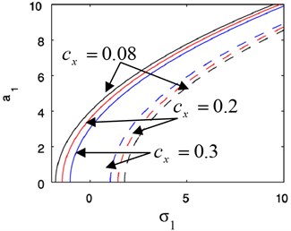
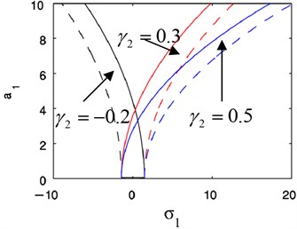
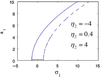
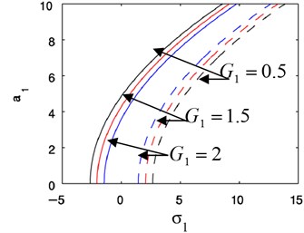
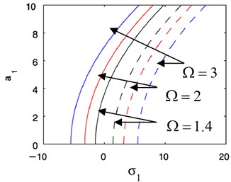
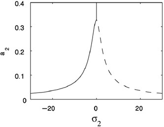
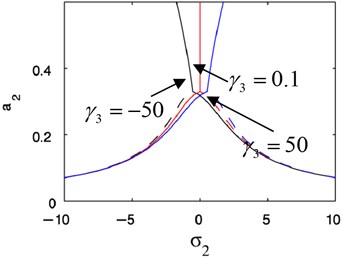
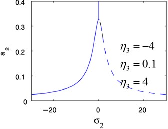
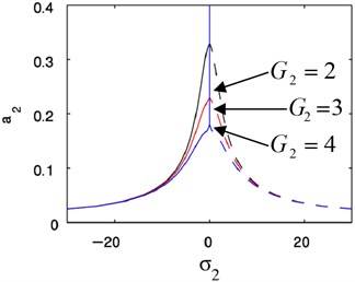
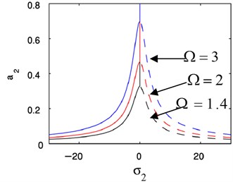
The frequency response Eqs. (38) and (39) are nonlinear algebraic equations of against and against respectively. These equations are solved numerically as shown in Figs. 4, 5. Some figures possess hard and soft effects. This bending leads to multi-valued solutions and jump phenomenon. There are stable (solid line) and unstable (dashed lines) solutions. The Table 1 shows all effects of the different parameters of the considered system.
Fig. 4Theoretical frequency response curves: cx= 0.2, γ2= 0.3, η2= 0.4, ωx= 2, Ω= 1.4, f1= 4, G1= 2
a)
b)
c)
d)
e)
f)
g)
h)
Fig. 5Theoretical frequency response curves: cy= 0.1, γ3= 0.1, η3= 0.1, ωy= 7.8, Ω= 1.4, Q= 4, G2= 2
a)
b)
c)
d)
e)
f)
g)
h)
6. Conclusions
The vibrations of second order nonlinear differential equations of a suspended cable system subjected to external, parametric and tuned excitation forces can be controlled via a negative linear velocity feedback controller. Multiple time scale perturbation technique is useful to determine approximate solutions for the differential equations describing the system up to second order approximation. To study the stability of the system, the frequency response equations are applied. The effects of the different parameters of the system are studied numerically.
From the above study the following may be fulfilled:
1) The worst resonance case of the system is the simultaneous sub-harmonic and combined resonance case , .
2) Negative linear velocity feedback active controller is the best one for the reported worst resonance case as it reduces the vibration dramatically.
3) The effectiveness of the best controller at the reported worst resonance case are about 2000 for x and 800 for , respectively.
4) The steady-state amplitudes of both modes are monotonic increasing functions in the parameters , , and while decreasing functions in the coefficients , , , and .
5) Also, for the nonlinear parameters , the steady-state amplitudes of both modes are making hardening and softening effects.
6) The nonlinear parameters , have no significant effects on the steady state amplitudes denoting the occurrence of saturation phenomenon.
References
-
Arafat H. N., Nayfeh A. H. Non-Linear responses of suspended cables to primary resonance excitations. Journal of Sound and Vibration, Vol. 266, Issue 2, 2003, p. 325-354.
-
Rega G. Non-Linear vibrations of suspended cables. Part I: modeling and analysis. Journal of Applied Mechanics Review, Vol. 57, Issue 6, 2004, p. 443-478.
-
Rega G. Non-Linear vibrations of suspended cables. Part II: deterministic phenomena. Journal of Applied Mechanics Review, Vol. 57, Issue 6, 2004, p. 479-514.
-
Zheng G., Ko J. M., Ni Y. O. Super-harmonic and internal resonances of a suspended cable with nearly commensurable natural frequencies. Nonlinear Dynamics, Vol. 30, Issue 1, 2002, p. 55-70.
-
Zhang W., Tang Y. Global dynamics of the cable under combined parametrical and external excitations. International Journal of Non-Linear Mechanics, Vol. 37, Issue 3, 2002, p. 505-526.
-
Chen H., Xu Q. Bifurcation and chaos of an inclined cable. Nonlinear Dynamics, Vol. 57, Issues 2-3, 2009, p. 37-55.
-
Benedettini F., Rega G., Alaggio R. Non-linear oscillations of a four-degree-of-freedom model of a suspended cable under multiple internal resonance conditions. Journal of Sound and Vibration, Vol. 182, Issue 5, 1995, p. 775-798.
-
Kamel M. M., Hamed Y. S. Non-linear analysis of an elastic cable under harmonic excitation. Acta Mechanica, Vol. 214, 2010, p. 315-325.
-
Abe A. Validity and accuracy of solutions for nonlinear vibration analyses of suspended cables with one-to-one internal resonance. Nonlinear Analysis: Real World Applications, Vol. 11, Issue 4, 2010, p. 2594-2602.
-
Srinil N., Rega G., Chucheepsakul S. Two-to-One resonant multi-modal dynamics of horizontal/inclined cables. Part I: theoretical formulation and model validation. Nonlinear Dynamics, Vol. 48, Issue 3, 2007, p. 231-252.
-
Srinil N., Rega G. Two-to-One resonant multi-Modal dynamics of horizontal/inclined cables. Part II: internal resonance activation reduced-order models and nonlinear normal modes. Nonlinear Dynamics, Vol. 48, Issue 3, 2007, p. 253-274.
-
Chen H., Zuo D., Zhang Z., Xu Q. Bifurcations and chaotic dynamics in suspended cables under simultaneous parametric and external excitations. Nonlinear Dynamics, Vol. 62, 2010, p. 623-646.
-
Ubertini F. Active feedback control for cable vibrations. International Journal of Smart Structures and Systems, Vol. 4, 2008, p. 407-428.
-
Zhao Y., Wang L. On the symmetric modal interaction of the suspended cable: three-to-one internal resonance. Journal of Sound and Vibration, Vol. 294, 2006, p. 1073-1093.
-
Wang L., Zhao Y. Nonlinear interactions and chaotic dynamics of suspended cables with three-to-one internal resonances. International Journal of Solids and Structures, Vol. 43, 2006, p. 7800-7819.
-
Zhao Y., Wang L. Non-linear planar dynamics of suspended cables investigated by the continuation technique. Engineering Structures, Vol. 29, Issue 6, 2007, p. 1135-1144.
-
Zhao Y., Wang L. Multiple internal resonances and non-planar dynamics of shallow suspended cables to the harmonic excitations. Journal of Sound and Vibration, Vol. 319, 2009, p. 1-14.
-
Sofi A., Muscolino G. Dynamic analysis of suspended cables carrying moving oscillators. International Journal of Solids and Structures, Vol. 44, 2007, p. 6725-6743.
-
Wang L., Rega G. Modelling and transient planar dynamics of suspended cables with moving mass. International Journal of Solids and Structures, Vol. 47, 2010, p. 2733-2744.
-
Huang K., Feng Q., Yin Y. Nonlinear vibration of the coupled structure of suspended-cable-stayed beam – 1:2 internal resonance. Acta Mechanica Solida Sinica, Vol. 27, Issue 5, 2014, p. 467-476.
-
Hieu N. Q., Hong K. S. Skew control of a quay container crane. Journal of Mechanical Science and Technology, Vol. 23, 2009, p. 3332-3339.
-
Kim D. H., Lee J. W. Model-based PID control of a crane spreader by four auxiliary cables. Proceedings of IMechE, Part C: Journal of Mechanical Engineering Science, Vol. 220, 2006, p. 1151-1165.
-
Masoud Z. Oscillation control of quay-side container cranes using cable-length manipulation. Journal of Dynamic Systems, Measurement, and Control, Vol. 129, 2007, p. 224-228.
-
Hamed Y. S., Amer Y. A. Nonlinear saturation controller for vibration supersession of a nonlinear composite beam. Journal of Mechanical Science and Technology, Vol. 28, Issue 8, 2014, p. 2987-3002.
-
Al-Qassab M., Nair S., Leary J. O. Dynamics of an elastic cable carrying a moving mass particle. Nonlinear Dynamics, Vol. 33, Issue 1, 2003, p. 11-32.
-
Kim J. H., Chang S. P. Dynamic stiffness matrix of an inclined cable. Engineering Structures, Vol. 23, Issue 12, 2001, p. 1614-1621.
-
Xu F., Wang L., Wang X., Jiang G. Dynamic performance of a cable with an inspection robot – analysis, simulation, and experiments. Journal of Mechanical Science and Technology, Vol. 27, Issue 5, 2013, p. 1479-1492.
-
Nayfeh A. H. Perturbation Methods. Wiley, New York, 1973.
Cited by
About this article

This project was supported by the deanship of scientific research at Prince Sattam bin Abdulaziz University under the research Project 2014/01/2110.
