A new controller design of electro-hydraulic servo system based on empirical mode decomposition

2.1. Brief introduction of EMD process

EMD method can decompose out every single intrinsic mode function (IMF) from high frequency to low frequency, which is self-adaption. Most of these IMFs have their own physical meaning. The process of EMD method is described in the following steps 1-3.

Step 1: Find out all the local maximum and minimum points. The local maximum and minimum points of original signal $x$ is defined in Eq. (1) and Eq. (2):

Step 2: Select a kind of interpolation method and employ it between all extreme points, then get the envelope curve $x_{max}\left(t\right)$ and $x_{min}\left(t\right)$.

Step 3: Calculate the difference $h\left(t\right)$ according to Eq. (3). If $h\left(t\right)$ does not satisfy Eq. (4), then repeat steps 1-3:

The first $h\left(t\right)$ satisfied Eq. (4) is the first IMF, let $I_1\left(t\right)=h\left(t\right)$, $r\left(t\right)={x\left(t\right)-I}_1\left(t\right)$, $r\left(t\right)$ be the original signal of next process round. Repeat steps 1-3, the rest of other IMF$I_2\left(t\right)$, $I_3\left(t\right)$, $I_4\left(t\right)$, …, $I_n\left(t\right)$ will be decomposed out. When $r\left(t\right)$ is a monotonic or constant series, this decomposition process will be terminated.

2.2. Optimizations of decomposition process

Review the whole process of EMD, the envelope curve is the key of decomposition. But the end point effect has significant influence on the decomposition [3], especially when the length of data is short. Many researchers have done a lot of work [9-12] to restrain the end point effect. To get a better filtering performance of short data, we make optimization of the EMD from four aspects as stated below.

Optimization 1: If the end point is the maximum or minimum point of the whole data section, then the end point will be treated as a local maximum or minimum point:

Optimization 2: The decomposition process may miss some turning points if the process follows the Eq. (1) and Eq. (2) strictly. And these missed turning points will reduce the effect of envelop curve as shown in Fig. 1. In this figure, $P_2$ and $P_{19}$ are two turning points, and they are not treated as local extreme points, so the envelop curves at point $P_4$ and $P_{18}$ are not complete: the max envelope curve is missed at point $P_4$ and the min envelop curve is missed at point $P_{18}$. At next process round, the value of point $P_4$ will change to $P_4^{\text{'}}$:

and the same thing will happen to point $P_{18}$.

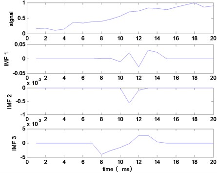
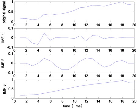
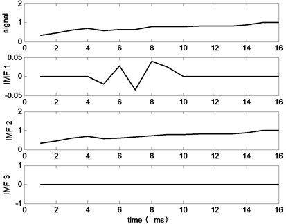
The decomposition result of Fig. 1 is shown in Fig. 2. We notice that the noise at point $P_4$ and $P_{18}$ is missed. Along with the further development of this decomposition process, $P_5$ and $P_{16}$ will also become 0. This effect will diffuse to the data center, then the data will be changed from $\left[x_1,x_2,x_3,\dots {,x}_{n-2},x_{n-1},x_n\right]$ to $\left[\mathrm{0,0},0,\dots 0,x_{n/2-p},\dots ,x_{n/2-1},x_{n/2},x_{n/2+1},\dots x_{n/2+q},0,\dots \mathrm{0,0},0\right]$. This means that the filtering effect only works in the data’s center area. The decomposition result under this situation is shown in Fig. 3, from this figure it’s easy to see that all the noise components (IMF1-IMF3) are not ideal.

Therefore, the turning points should be included in the definition of local extremely points. The maximum point of turning point is redefined as Eqs. (5)-(6), and the minimum point of turning point is redefined as Eqs. (7)-(8);

Fig. 1Effect of turning point on envelope (a)

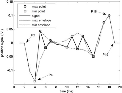
Fig. 2Effect of turning point on envelope (b)

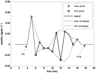
Fig. 3The decomposition result without considering turning points

After extending the definitions of local maximum and minimum points, the new max points, min points and envelope curves in Fig. 1 are shown in Fig. 4 and Fig. 5. The envelope curves can be obtained by using three spline interpolation method. With considering the point $P_2$ and $P_{19}$, the max envelop curve and min envelope curve become complete. The value of point $P_4$ changes to $P_4^{\text{'}\text{'}}$: ${P_4^{\text{'}\text{'}}=P}_4-{(P}_{4max}+P_{4min})/2\ne 0$. At next process round, the decomposition result is shown is Fig. 5. In Figs. 4 and 5, we can notice that the diffusion effect of data changing into 0 no longer exists.

After using these revised definitions, the decomposition result of the signal in Fig. 3 is shown in Fig. 6. In this result, IMF1 and IMF2 are the noise components, IMF3 is the useful signal. Compared Fig. 6 with Fig. 3, the new filter works better, which means the optimization 2 is necessary and effective.

Optimization 3: The envelop curve may have overshoot or undershoot when the span between two local extreme points is too larger than others. This situation is shown in Fig. 7. As shown in this figure, the span between point $P_2$ and $P_{53}$ is $d_1$, $d_1=\mathrm{}$53$-$2$=$51. The other spans are $d_2$ to $d_4$, $d_2=\text{68}-\text{53}=\text{15}$, $d_3=\text{77}-\text{68}=\text{9}$,$d_4=\text{97}-\text{77}=\text{20}$, the average value of these spans is $d_{mean}$, $d_{mean}={(d}_1+d_2+d_3+d_4)/4=$23.75, $d_1>{\text{1.5}d}_{mean}$. The undershoot (between point $P_2$ and $P_{53}$) of envelope curve will have a significant impact on the results. In this example, the value of local max points’ envelope curve is smaller than local min points’ envelope curve, which will introduce errors into final result. In this undershoot section, the envelope curve is ought to be the signal itself, the correct calculation process should be:

implying that there is no noise in the data of this section. But due to this undershoot, the calculation result becomes $P_i^{\text{'}}=P_i-(P_{imax}+P_{imin})/2\ne 0$, indicating that the process will introduce some error noises into result.

Fig. 4The envelope effect with considering turning points (a)

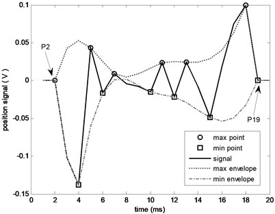
Fig. 5The envelope effect with considering turning points (b)

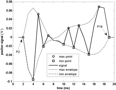
Fig. 6The decomposition result with considering turning points

In order to avoid this situation, interpolation method could be an outstanding solution. Firstly, the average span $d_{mean}$ of $[d_1,d_2,d_3,\dots ,d_m]$ can be calculated by Eq. (9), in which $d_i$ represents the span between two local extreme points $P_p$ and $P_q$, $d_i=p-q$. Secondly, find out the maximum span according to Eq. (10) and (11). Thirdly, insert points in the data section which has the maximum span. If the data is $\left[x_1,x_2,x_3,\dots ,x_N\right]$ and local extreme points are $[e_1,e_2,e_3,\dots ,e_{n+1}]$, and the max span is between $e_i$ and $e_j$, $1\le i<j\le n+1$, so the exteme points will change to $[e_1,e_2,e_3,\dots ,e_i,{x_{i+1\bullet d_{mean}},x_{i+2\bullet d_{mean}},\dots ,x_{i+t\bullet d_{mean}},e_j,\dots ,e}_{n+1}]$ after interpolation, in which $t=j-i/d_{mean}$, $t\in N$:

in which $N$ is the length of data, $n$ is the number of span.

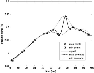
After applying this interpolation method, the envelop curve in Fig. 7 has been improved which is shown in Fig. 8.

Fig. 7The decomposition result after considering turning points

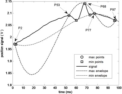
Fig. 8The envelop curve after interpolation

Optimization 4: In order to improve calculation efficiency and reduce operation time, a termination condition Eq. (12) is added. Because in some cases, the noise components are just in the first few IMFs, the filtering result will be inaccurate if the decomposition process runs to the final step ignoring Eq. (12). For example, if the noise components are $[{IMF}_1,\dots ,{IMF}_i]$, the other components $[{IMF}_{i+1},\dots ,{IMF}_n]$ are useful signals. The original signal is $s$:

If the filter takes $[{IMF}_{i+1},\dots ,{IMF}_n]$ as noises, then the signal after filtering will be $s^{\text{'}}$:

This situation is shown in Fig. 9, only $IM{F}_1$ is the noise component, $IM{F}_2$ is useful signal, and the filter takes the other IMFs as noise components, the filtering result will be all zeros.

To avoid this situation, Eq. (12) is employed to judge the similarity between the original signal and the decomposition component. If the decomposition result is similar to the original signal, the decomposition process should be stopped:

in which $X_i$ is the original signal, $I_i$ is the $IMF$ component.

Fig. 9The noise component is only in IMF1

3.1. The order of noise components

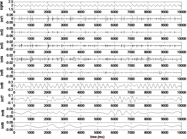
Before the start of decomposition process, the order of noise components needs to be determined. Decompose the acquired data of electro-hydraulic servo system by using EMD method, and the result is shown in Fig. 10. The noise components are mainly in the first few components $IM{F}_1$-$IM{F}_5$, therefore, the process should be ended at $IM{F}_5$. The signal $x\left(t\right)$ becomes $y\left(t\right)$ after filtering, $y\left(t\right)=x\left(t\right)-{IMF}_1-{IMF}_2-{IMF}_3-{IMF}_4-{IMF}_5$.

Fig. 10The decomposition result

3.2. The length of filtering window

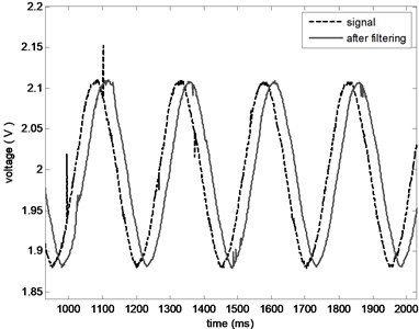
The length of filtering window is vital to filtering process. On one side, the longer the window is, the more information it contains. On the other side, the longer the window is, the more time and the bigger phase delay it takes. Therefore, a trade-off between these two sides is necessary. Compare the results of length 20 and length 50, which are shown in Fig. 11 and Fig. 12, respectively, the length of this system is determined to 50.

3.3. The properties of the filter

Property 1: This new filter is self-adaptive, because this filter works in time domain and the decomposition process is based on the characteristic of the signal itself. When we design this new filter, the interpolation method, the orders of noise and the length of filter window are priorities need to be considered, the frequency of the signal and noise is no longer the main parameters for the design of this filter.

Property 2: The phase delay of this new filter is fixed. For the traditional digital filter, the phase delay changes with the change of input signal’s frequency. If the central point of the filtered data is taken as the result of the filter and the data length is $n$. The data in filter window is $\left[x_1,x_2,x_3,\dots ,x_n\right]$, at next sampling time the data will change to $\left[x_2,x_3,x_4,\dots ,x_{n+1}\right]$, when sampling point $x_{n+1}$ moves to the center of filter window, the data becomes $\left[x_{n-n/2-1},x_{n-n/2},{\dots ,x_n,x}_{n+1},x_{n+2},\dots ,x_{n+n/2}\right]$. So the phase delay is $n/2\bullet t$, where $t$ is the sampling time. It’s clear that the phase delay is not related to the frequency of the input signal, and only related to data length $n$ and sampling time $t$.

Fig. 11The decomposition result when the window length is 20

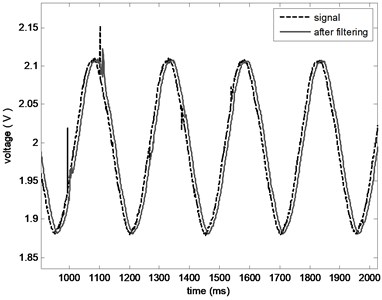
Fig. 12The decomposition result when the window length is 50

4.1. The compensation of phase delay

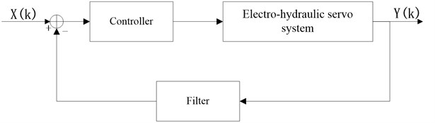
The picture of practical object and the control block diagram of electro-hydraulic servo system are shown in Fig. 13 and Fig. 14, respectively. The presence of the filter in feedback will have some influences on amplitude and phase. The phase delay of traditional filter like Butterworth filter and Chebyshev filter always grows larger while frequency becomes higher. But the phase delay of this new improved HHT filter is only related to the length of filtering window $n$, and maintains $n/\text{2}$ sampling periods delay. Based on this feature, the phase delay could be compensated in controller.

Fig. 13The picture of the practical object

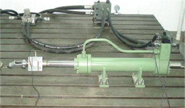
Fig. 14The system block diagram

This electro-hydraulic servo system is a position control system, and its transfer function can be obtained by using system identification. The form of transfer function is shown in Eq. (13):

in which $A\left(z^{-1}\right)=1+a_1{z}^{-1}+a{z}^{-2}+a_3{z}^{-3}$, $B\left(z^{-1}\right)=b_0+b_1{z}^{-1}+b_2{z}^{-2}+b_3{z}^{-3}$. $z^{-n/2}$ in Eq. (13) shows that there is a $n/2$ orders delay in system. To compensate this delay, the input $X\left(k\right)$ becomes $X\left(k+n/2\right)$, and then the change of output $Y\left(k\right)$ is shown in Eq. (14):

After compensation, the phase delay is only related to system itself.

4.2. Stability analysis of controller

The property 2 of this new filter means that a delay link is added to the system. The system’s open loop transfer function will be changed from $B\left(z^{-1}\right)/A\left(z^{-1}\right)$ to $z^{-n/2}B\left(z^{-1}\right)/A\left(z^{-1}\right)$. If the input signal is $X\left(k+n/2\right)$, then the output signal $Y\left(k\right)$with noise $N\left(k\right)$is:

The noise after filtering becomes $N^{\text{'}}\left(k\right)$, $N^{\text{'}}\left(k\right)=N\left(k\right)-e\left(k\right)$, $e\left(k\right)$ is the error between original noise and filtering result. Because the real filter cannot achieve the ideal effect, the error always exists. The system’s output after filtering is $Y^{\text{'}}\left(k\right)$, $Y^{\text{'}}\left(k\right)=\left(B\right(z^{-1})/A\left(z^{-1}\right))X\left(k\right)+e\left(k\right)$. So this new controller’s stability is only related to system itself, and does not introduce additional stability influence.

Fig. 15The effect comparison chart at 2 Hz

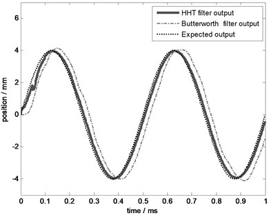
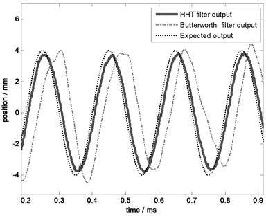
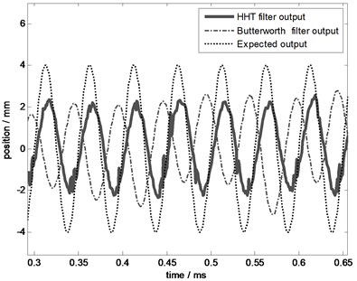
Fig. 16The effect comparison chart at 5 Hz

4.3. The control result

Apply this new controller in system and test the control performance at frequency 2 Hz, 5 Hz, 10 Hz, and 20 Hz. To illustrate the practicability and the superiority of this new controller, take Butterworth filter (Low pass filter, with pass band 0-20 Hz, pass band attenuation no more than 3 dB, the attenuation of 150 Hz at least 60 dB) as a comparison filter. The comparison results are shown in Figs. 15-18, illustrating that the control error of this new filter is less than Butterworth filter especially at high frequency.

Fig. 17The effect comparison chart at 10 Hz

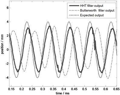
Fig. 18The effect comparison chart at 20 Hz