Abstract
Hydraulic system lubricating oil is subject to serialized Variable Static Loads (VSL) following-up performance. An improved Self-Turbulent Flow (STF) algorithm, based on the real-time acquisition and monitoring of Lubricating Oil Static Pressure (LOSP) in hydraulic system to simulate VSL, is proposed. In this topic, a mathematical model of the Electro-Hydraulic Servo (EHS) control system for LOSP acquisition is presented, and the STF controller is designed for numerical analysis. The Self-Anti-Disturbance (SAD) control strategy for LOSP of EHS system is discussed, which is used for quadratic optimization, pole placement, PID and STF control, and the LOSP simulation model of STF control is constructed by SIMULINK module. Numerical simulation results indicate that the overshoot is significantly reduced. The proposed SAD control algorithm is verified by experiments, and the LOSP acquisition followability and monitoring accuracy are greatly improved. Toward this goal, a variable hydraulic LOSP acquisition and monitoring can be effectively and stability adjusted by pre-designed EHS control system in the field of power hydraulic fluid lubrication.
Highlights
- An improved Self-Turbulent Flow (STF) algorithm for Lubricating Oil Static Pressure (LOSP) in hydraulic system to simulate Variable Static Loads (VSL) following-up performance is proposed.
- A mathematical model of the Electro-Hydraulic Servo (EHS) control system for LOSP acquisition is presented.
- The STF controller is designed for numerical analysis.
- The LOSP simulation model of STF control is constructed by SIMULINK module.
- The proposed SAD control algorithm is verified by experiments.
- The LOSP acquisition followability and monitoring accuracy are greatly improved.
1. Introduction
A hydraulic system typically transfers a fluidic medium from one hydraulic element to another, capable of delivering serialized variable hydraulic loads to a contact lubrication area [1, 2]. The extremely core components for a hydraulic system are an actuator or hydraulic motor, different control valves, accumulators, and a hydraulic pump [3, 4]. The variable LOSP acquisition and SAD control strategy of the entire hydraulic system are key links, and which are adversely constrained by the VSL of different hydraulic components [5]. The acquisition efficiency is less with the increase of hydraulic components number and hence weaken the control strategy effectiveness of the hydraulic system. As a result, a hydraulic system optimal design may maximize the timeliness of the control strategy [6-8]. When it is mandatory restraint to play dual functions by a hydraulic system, the hydraulic components number is usually more [9, 10]. Hence, the SAD function affecting the overall control strategy of the s hydraulic system is relatively higher, and the key corrective measures is to reduce the connection of hydraulic components or seek to optimize the control link design [11, 12]. In this investigate, a new hydraulic control system strategy is bound to be proposed to verify the simulation results of LOSP acquisition and monitoring. At present, others have studied state stochastic linear quadratic optimal control, proposing that the optimal control strategy is a piecewise affine function of the system state [13, 14]. Consideration should be given to the controllable high precision of hydraulic systems that have been widely used in many industries. The hydraulic system can provide a large rigidity LOSP, which is a prominent advantage and extremely necessary for the above description. The bottleneck of high-precision control of hydraulic system is nonlinear characteristics and modeling uncertainty, to be specific, the parametric quantification uncertainty and Self-Anti-Disturbance (SAD) are the main obstacles now. Therefore, an optimal control strategy for parameter uncertainty handling and SAD improvement is realized synergistically. A new method for inverse resonance assignment and regional pole assignment for linear time-invariant vibrational systems is presented [15, 16]. Currently, although many scholars have used quadratic optimal control and pole configuration to solve related practical engineering problems, this control method has not been introduced into the optimization research of hydraulic lubrication system yet [17, 18]. There are many research results on the above-mentioned special issue, and most of the current controllers are mainly anti-interference, represented by adaptive robust control [19, 20]. The hydraulic system has applied a variety of advanced control methods to ensure the transient performance of the hydraulic system and the specified steady-state performance. An Electro-Hydraulic Servo (EHS) control system for LOSP acquisition has been widely used in many fields of modern industry [21, 22]. Considering the uncertainty of the EHS system model, for important equipment such as the hydraulic system of warship power rear transmission system, the traditional control algorithm can no longer meet the requirements of the warship's hydraulic system. In this argument, the improved Self-Turbulent Flow (STF) controller for hydraulic system state estimation based on EHS mathematical model is an effective solution for LOSP acquisition and monitoring [23, 24]. The precise control of EHS system for LOSP through SAD strategy has been studied in many aspects in academia, but it has not been applied in practice only at the theoretical level. The active disturbance rejection control algorithm to optimize the performance of the hydraulic system is adopted, and the specific servo control technical structure and regulation error feedback mechanism is revealed [25]. It is pointed out that the integrator series structure of hydraulic servo control system can correspond to linear or nonlinear system under the condition of feedback. By considering the system function as state feedback, a scalable state controller is proposed, which can use servo feedback control the hydraulic system [26, 27]. To be more specific, a LOSP simulation model of STF control algorithm adjusted by pre-designed EHS system is introduced to simultaneously deal with parameter uncertainties and time-varying disturbances demonstrate in hydraulic system. The fly in the ointment is that time-varying disturbances cause asymptotic loss of hydraulic servo system stability, although the desired LOSP acquisition and monitoring performance can be guaranteed at low feedback gains [28, 29]. For a stochastic hydraulic system, when multiple heterogeneous disturbances exist simultaneously, the closed-loop system is asymptotically bounded on the mean square, and with the disappearance of the additive disturbance, the equilibrium is globally asymptotically stable in probability. If the uncertainty terms can be linearly parameterized, an adaptive control scheme with the addition of a power integrator technique is proposed, and the mismatch disturbance is estimated by the designed disturbance controller [30, 31]. The global asymptotic stability of the closed-loop system is guaranteed only when the perturbation is constant. Fuzzy logic systems are used to approximate unknown nonlinear functions, and nonlinear disturbance controllers are used to estimate unknown external disturbances. In this work, all signals are semi-globally consistent eventually bounded, and local neighborhood inclusion errors can converge to the prescribed bounds. The hydraulic actuator adopts a high-order sliding mode controller, and the control gain is adaptive online. The proposed controller still cannot achieve asymptotic following control performance. In this paper, a disturbance controller for pump-controlled hydraulic system based on error function is developed, and asymptotic following control is realized. The desired asymptotic LOSP control can also be achieved by using a jitter-free robust finite-time output feedback control scheme. Failure to consider parameter uncertainties results in an overburdened learning burden for the disturbance controller, and the hydraulic system servo performance deteriorates when the considered control device is subject to severe parameter uncertainty.
2. EHS control modeling of hydraulic system
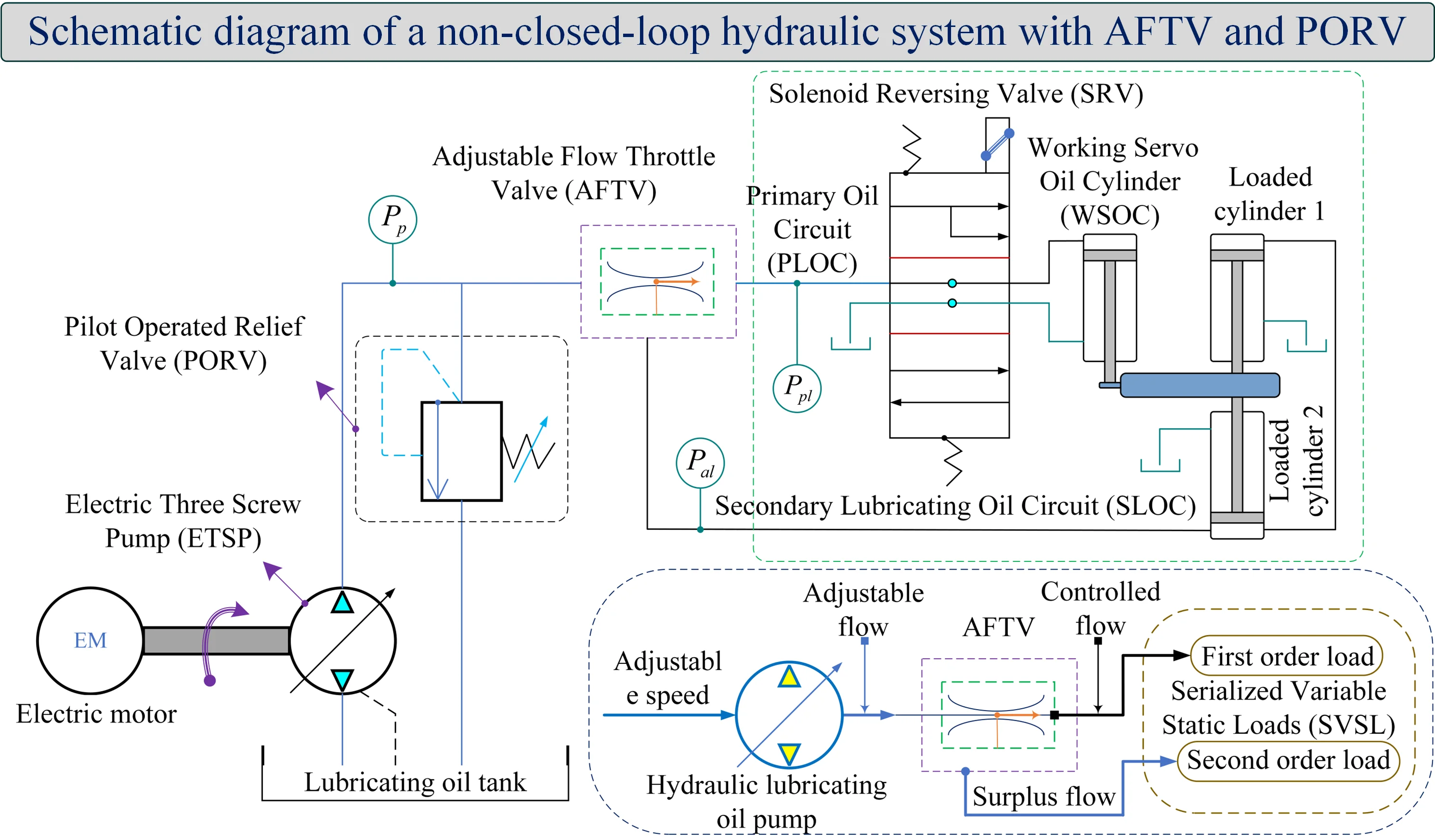
Hydraulic systems transmit power using a fluidic medium. It converts the mechanical power from an engine or an electric motor to hydraulic power by rotating the shaft of a hydraulic pump. The hydraulic pump provides flow to the control valve, which directs the same flow to the hydraulic actuator and converts hydraulic power back to mechanical power. In this sub-project, two different non-closed-loop hydraulic systems are presented, refer to Fig. 1, respectively, which are determined to analyze the function of an Adjustable Flow Throttle Valve (AFTV). The AFTV is preferred over the choice of Pilot Operated Relief Valve (PORV) to perform two different performances simultaneously. Also, is more suitable for providing a constant flow whenever the input flow has a fluctuating nature. This stated novel idea is preferable in JC power rear transmission systems to generate stable output power and torque.
Fig. 1Schematic diagram of a non-closed-loop hydraulic system with AFTV and PORV
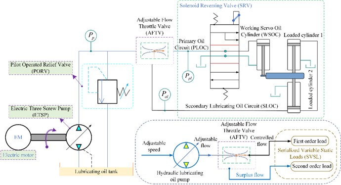
In Fig. 1, a lubricating oil hydraulic pump with serialized VSL rigidity is supplied a variable flow to the AFTV. The AFTV is responsible for two different loads, namely a first-order load and a second-order load of the hydraulic system. The AFTV directs the Electric Three Screw Pump (ETSP) flow towards the primary and secondary loads of the hydraulic system. Depending on the load of the hydraulic system, the ETSP flow is regulated by controlling the movement of the pump shaft. A PORV is installed between the ETSP and AFTV to maintain the normal system pressure and thus acts as a safety valve. In the present study, the dynamic model of the hydraulic system is not taken seriously, as the central issue is to analyze the performance of the AFTV using hydraulic mechanism. The scheme proposes to obtain constant power and torque from the JC Gear Transmission System (GTS) to JC Controlled Pitch Propeller (CPP) adopting a AFTV and two PORVs. In this case, a hydraulic ETSP is used to provide variable flow to the AFTV. The Primary Lubricating Oil Circuit (PLOC) of AFTV is tunable while per stable load conditions and assembled at a threshold. Once above the given flow from the ETSP to maintain a steady load, additional given flow from the ETSP will be allowed through the auxiliary port of PORV. The surplus flow is returned to the lubricating oil tank in the Secondary Lubricating Oil Circuit (SLOC) of the hydraulic system and stored in the hydraulic accumulator. Contrary to the above, if the given flow from the pump to the AFTV is lacking, the flow is unable to satisfy the hydraulic motor to provide the required working flow to maintain the constant speed of the GTS and CPP.
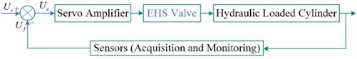
In this case, the EHS control valve receives a signal from the on/off controller. Thereafter, the stored oil fluid from the accumulator compensates the supplied flow to the hydraulic motor, which helps maintain constant speed and torque of the GTS/CPP when the ETSP output flow is undersupplied. The hydraulic system discussed above can replace hydraulic power transmission in turbine applications to obtain the required stable power elements therefrom. The schematic diagram of the EHS control system is shown in Fig. 2. The block diagram of the hydraulic control system is shown in Fig. 3.
Fig. 2Schematic diagram of the EHS control system
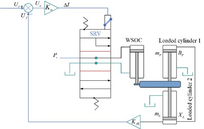
Fig. 3Block diagram of the hydraulic control system
The hydraulic control valve flow equation, the cylinder flow continuity equation and the force balance equation between the cylinder and the load are established respectively:
where, is VSL flow (m3/s), denotes supplied flow gain factor, represents the displacement of EHS valve spool (mm), is pressure-flow gain factor, is VSL pressure (Pa), denotes an effective working area of hydraulic servo cylinder (m2), is the displacement of the piston rod of the hydraulic cylinder (mm), represents the total leakage coefficient of hydraulic cylinder, is total compressed volume (m3), is effective bulk elastic modulus, is VSL flow damping factor, is VSL flow quality (kg), is VSL flow elastic stiffness.
The above equations can be expressed by Laplace transform as:
The control system deviation voltage signal equation and feedback link pressure sensor equation are established respectively:
where, is input voltage signal (V), is feedback voltage signal in the system link (V), is sensor pressure gain amount (V/N), is hydraulic servo cylinder output force (N).
If only the static performance of the amplifier is considered, its output current is:
where, denotes servo amplifier gain amount (A/V). The EHS valve transfer function is expressed as:
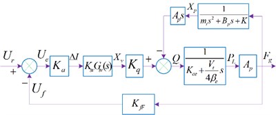
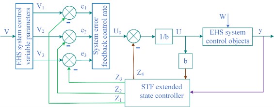
where, is an EHS valve displacement (mm), is an EHS valve hydraulic gain amount (m3/s∙A), then . Based on the above formulas, the hydraulic system block diagram is shown in Fig. 4, where holds.
Considering the complex dynamic performance model of EHS system, there are fifth-order, fourth-order and third-order functions respectively. Moreover, the response speed of the EHS valve is fast, only the static performance is considered here, and it is directly set as the proportional link, then the mathematical model of the hydraulic system in this paper is simplified as:
The parameter assignment and simplification of Eq. (9), and the transfer function is derived, which can be regarded as:
In this scheme, the classical PID is optimized through the Self-Turbulent Flow (STF) control algorithm, and the specific structure of the STF controller is designed. The Simulink module is used to simulate the control system. After comparative analysis, the changing laws of the response curves of the four control strategies are proposed.
Fig. 4Hydraulic system block diagram with EHS control
3. Simulation analysis of optimal control strategy
The Self-Anti-Disturbance (SAD) control strategy for LOSP of EHS system is discussed in detail, which is used for quadratic optimization, pole placement, PID and STF control, and the LOSP simulation model of STF control is constructed by SIMULINK module.
3.1. Quadratic optimal control analysis with linearity
The principle of optimal control is to find a control variable that has a small value and can satisfy the minimum system error , so that the output of the system quickly follows the input and the energy consumption is low. The minimum value of the index can be obtained from the Pontryagin principle, and the essence of the quadratic optimal control is the approximation of the feedback of the original system. In this study, using the feedback of the optimal regulator to approximate the optimization, the simplified optimal control rate can be expressed as:
The algebraic equation for the Riccati matrix can be given as:
where, denots the EHS system matrix, is the control matrix of the EHS system, and are the weighting matrices of the EHS system, herein , 0.0001, is the numerical solution of the equation.
Therefore, the optimized system matrix can be described as:
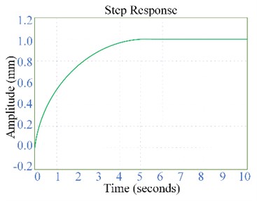
Using Matlab to simulate the transfer function under quadratic optimal control, the step response curve of the EHS system after quadratic optimal control with linearity is revealed, as shown in Fig. 5. It can be seen from Fig. 5 that the EHS control system can reach stability in 4.8 s. After the control system undergoes secondary optimization control, the stabilization time is shortened by 15.3 s, and the control performance is greatly improved, but unfortunately the time is relatively long.
Fig. 5Step response curve of the EHS system after quadratic optimal control with linearity
3.2. Pole optimized configuration
Introducing the state feedback gain matrix , then the characteristic polynomial can be expressed as:
The core content of analyzing the performance of the control system is to determine the dominant pole, where the effect of the far pole is ignored. Therefore, the EHS control system is considered to be equivalent to a second-order control system containing a main pair of poles. Determining the location of the expected dominant pole from the representation of the dynamic indicators % and , it will be as follows:
where, % represents the maximum overshoot, is the damping (0 1). Assuming that the allowable error of the EHS control system is set to 5 %, there is:
where, is the adjustment time (s), denots the undamped frequency (rad/s). The expected dominant pole of an EHS system can be expressed as:
where, are the EHS system expects to dominate the poles. Considering that the maximum overshoot of the EHS control system is limited to % ≤ 5 %, and the adjustment time is set to 0.5 s, the expected dominant poles ( and ) of the EHS system can be given by the following Eq. (18). Analyzing this equation, the following settings are specified:
Herein, the clear value is 0.707, 6.0 = 6, then there is:
Let the third pole be set, so the following expression is:
Established by , and then obtain the following expression:
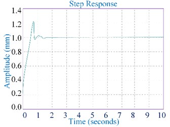
Fig. 6 shows the step response curve of the pole optimal configured EHS control system obtained by the Simulink module simulation. As can be seen from Fig. 6, the EHS system can be stabilized within 1.3 seconds. After the EHS control system is optimized by the pole configuration, the stabilization time is shortened by 20.3 seconds, and the control performance is significantly improved, but the overshoot phenomenon occurs prematurely.
Fig. 6Step response curve of the EHS system after pole optimal configured control
3.3. Simulation analysis of classical PID control
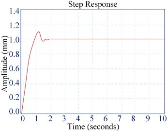
The simple structure and convenient parameter calibration of classical PID control make it widely used in many fields. In this chapter, the proportional coefficient is firstly determined, and the integral constant and differential constant are set to zero. The proportional gain gradually increases from zero until the response curve oscillates, and then the value decreases slowly until the oscillation stops, 30 %-70 % of the proportional gain is used as the system proportional coefficient, and 60 % is taken in this study. The proportional coefficient is determined, and the larger value is taken as the initial value of the system integral constant. After several adjustments, the system stops oscillating, and 150 %-180 % of the integral constant is taken as the final value of the integral constant of the system, which is set as 165 %. In the case of EHS system output force, the differential constant is usually chosen to be 0. The parameters of the classical PID controller are selected as 11.17, 63.11, 0. The step response curve of classic PID control of EHS system simulated by Simulink is shown in Fig. 7.
In Fig. 8, the EHS system has some improved performance through PID control. When a unit step signal is input, the EHS system tends to a stable state within 1.55 s, and its input and output signals have good matching performance, but the EHS system is also accompanied by a certain amount of overshoot.
Fig. 7Step response curve of the classic PID control of the EHS system simulated by Simulink
3.4. Simulation analysis of SAD control
To further improve the control effect of the control system, on the basis of the SAD control algorithm, the classical PID is comprehensively optimized, and the optimal scheme of the overall performance of the system is proposed, and the SAD controller is analyzed and designed in combination with the specific structure. The designed block diagram of the proposed SAD third-order controller in this paper is shown in Fig. 8.
Fig. 8Designed block diagram of the proposed SAD third-order controller
The SAD controller consists of three modules, the control parameter Following Differentiator (TD), the error feedback Extended State Controller (ESC) and the EHS Control Law (CL). Based on the system state space expression, the controlled object is set to be third-order, where the TD is third-order, and the ESC is fourth-order. Seeking to improve the dynamics of this control system, use state feedback to configure the desired poles. If the zero-point configuration of the control system can be realized, the dynamic performance of the control system can be improved. However, the zero point configuration needs to use the differential signal. The differential cannot filter out noise, nor is it used for zero point configuration, while the following differential can filter out the noise well, and the differential signal is zero point configuration. The TD follows a given signal and obtains its differential equation. The transition process is arranged by TD to prevent the overshoot caused by the sudden change of the given signal, so that the controlled objects approach the target smoothly, thereby improving the stability of the control system. By eliminating the poles of the system with the configured zeros, the system can be viewed as a control system close to unity. This sets the string level object to the following expression:
Assuming that is known, the virtual control volume is:
The above Eq. (21) can be written as:
Once the virtual control quantity is clarified, the actual control quantity acts as:
where, and are polynomials.
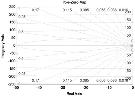
Fig. 9Zero-pole diagram of the controlled object exported by Matlab
The virtual control volume is determined by applying a improved controller design of Self-Turbulent Flow (STF) algorithm approach to the control subsystem , which thus allows for a certain range of uncertainties to exist. Assuming that the mathematical model of the controlled object contains zeros and poles, its general form can be described as:
Set the virtual control quantity , then the system becomes , then the actual control quantity becomes . If the controlled object conforms to the minimum phase system, the belongs to a stable polynomial and is known. The SAD controller can be used to determine the virtual control quantity , and the actual control quantity can be obtained by solving the system with as the input. Through the above analysis, the zero-pole diagram of the controlled object is derived using Matlab, as shown in Fig. 9.
As can be seen from Fig. 9, the system model has no zeros and poles in the positive part of the complex plane and is considered as a minimum phase system. In this case, the virtual control variable is determined by the active disturbance rejection controller, and is used as the input to solve the system to obtain the actual control variable. The transfer function of the control system is known to satisfy the cubic polynomial . The parameters , and are known, and the STF algorithm of the third-order TD differentiator is written as:
where, is a fast factor, denotes the sampling step size.
The error feedback Extended State Controller (ESC) follows the output of the control system, monitors the state of each stage of the research object and the total perturbation of the EHS system in real time, and then compensates the perturbation accordingly. If the system suffers from unknown disturbances, the control object is uncertain. This indeterminate object is expressed as:
where, is system unknown function, is the unknown perturbation, is a control gain, is the system input, is the system output.
The error feedback ESC in this paper is fourth-order. Under linear conditions, the fourth-order ESC algorithm of the control system is written as:
where, , , , are the ESC parameters, is the feedback error term.
The transfer relationship from input to output of the error feedback ESC is expressed as:
In the control system, the ESC contains four output variables, follows the system output , follows , follows , and follows the system integral disturbance, and the disturbance is compensated by the feedforward method. In order to achieve a predetermined estimation accuracy, a larger gain coefficient is selected, that is, a larger value of the gain coefficients , , , is required to satisfy the high-gain ESC mode. Based on the four optimization methods and control strategy system models of classical PID control, quadratic optimization control, pole configuration and SAD, the EHS system is simulated by Simulink, and the step response curves of the unit step signal under the four control strategies are compared and analyzed, as shown in Fig. 10.
Fig. 10Step response curve of unit step signal under four control strategies
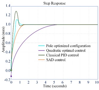
In Fig. 10, the SAD performance is the most stable after the system is optimized. The response speed of PID is 0.6 seconds slower than that of SAD control, and the response is accompanied by a large amount of overshoot. The response time of the pole configuration is 0.3 seconds longer than that of the SAD control. Compared with the PID control, although the overshoot is significantly reduced, the overshoot still exists. Both quadratic optimal control and SAD control do not have overshoot, but the response time of SAD control is 4.8 seconds shorter than that.
4. Experimental analysis
4.1. Experiment setup
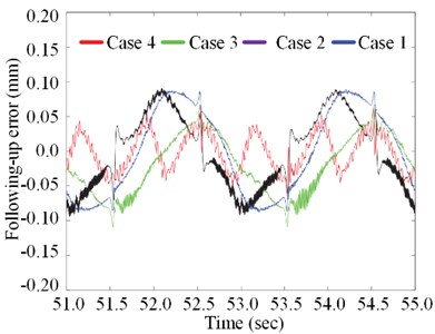
To verify the effectiveness of the proposed four control strategies, a hydraulic platform has been established, which is referred Fig. 11 for details. For testing the proposed controllers, the experimental following-up error performance is shown by quantitative acquisition and monitoring in this section. The verification platform consists of a hydraulic system including a double-rod hydraulic cylinder, a linear encoder (accuracy class ±5.0 μm) for position and velocity information, two oil pressure sensors (accuracy class 0.1 MPa) for measuring differential pressure, a servo valve (rated flow rate 18 L/min at 0.6 MPa) with a bandwidth higher than 120 Hz, drive shaft, mass load 50 kg, hydraulic supply with 1.0 MPa, and measurement and control system. The measurement and control system consists of monitoring software, real-time control software, A/D card (Advantech PCI-1716), D/A card (Advantech PCI-1723), counter card (Heidenhain IK-220), all these cards are 16-bit. The monitoring software is programmed with NI LabWindows/CVI, and the real-time control software is compiled with Microsoft Visual Studio 2005 plus Ardence RTX7.0. Ardence RTX 7.0 is used to provide a real-time working environment for real-time control software under Windows XP operating system. To implement the proposed controller and other comparison controllers defined below, the discretized C++ code was programmed. The control sampling time for the control is 0.4ms. The following-up errors of the four control strategies within 1.0s are revealed in Fig. 12. The following-up errors of the four control strategies within 4.0s are revealed in Fig. 13. Where, Case1 represents the pole optimized configuration, Case2 represents the quadratic optimal control, Case3 represents the classical PID control, Case4 represents the SAD control.
In Figs. 12 and 13, the following-up performance of the Case 4 controller is better than that of the others, which is clearly evident. It is also noted that the following-up performance of the Case 2 controller is relatively weak, which indicates that the parameter uncertainty has a great influence on the high frequency band of the controller. Similarly, the following-up performance of the conventional PID controller (Case 1) is the least ideal compared with that of the others.
Fig. 11The EHS system experiment platform
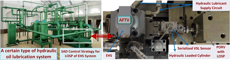
Fig. 12Following-up errors within 1.0 s
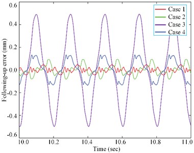
Fig. 13Following-up errors within 4.0 s
4.2. Discussion of the results
From these results above, especially looking to Figs. 12 and 13, is it certain that it is possible to conclude that, the following-up of the controller of Case 3 is greatly in-creased compared with that of Case 1 and Case 2. An improved STF algorithm is introduced into the EHS system with LOSP optimized for the SAD control strategy, which is a novel move. Another interesting consideration is the comparison of the gains of the Cases, it is possible to state that the following up performance of the Case 4 controller is better than that of Case 3. On the other side, it is verified that the variable hydraulic LOSP acquisition and monitoring proposed in this paper can be effectively and stability adjusted by a pre-designed EHS control system.
5. Conclusions
The motivation for this study is the serialized Variable Static Loads (VSL) following-up performance challenge presented in hydraulic systems to develop a Self-Anti-Disturbance (SAD) control optimal strategy for Lubricating Oil Static Pressure (LOSP) of Electro-Hydraulic Servo (EHS) system that is efficient at the performance level and asymptotically stable at the theoretical level. To this purpose, an improved Self-Turbulent Flow (STF) algorithm is introduced, which can simultaneously deal with parameter uncertainty and time-varying disturbances. Based on the proposed algorithm, the VSL asymptotic stability of the hydraulic system is achieved. Considering that the dynamics of these valves such as Adjustable Flow Throttle Valves (AFTV) and Pilot Operated Relief Valves (PORV) are often overlooked in hydraulic system lubrication design, one of the future studies is to investigate EHS valve dynamics modeling techniques to improve optimal dynamic following-up performance. In addition, considering the practical application reasons such as volume/cost/weight, the fly in the ointment is that the full state feedback cannot be realized in this study, which will prompt further discussions on the output feedback control of the hydraulic system.
References
-
S. Kumar, K. Dasgupta, and S. K. Ghoshal, “Fault diagnosis and prognosis of a hydro-motor drive system using priority valve,” Journal of the Brazilian Society of Mechanical Sciences and Engineering, Vol. 41, No. 2, pp. 1–18, Feb. 2019, https://doi.org/10.1007/s40430-019-1572-7
-
H. Ding, Y. Liu, and Y. Zhao, “A new hydraulic synchronous scheme in open-loop control: Load-sensing synchronous control,” Measurement and Control, Vol. 53, No. 1-2, pp. 119–125, Jan. 2020, https://doi.org/10.1177/0020294019896000
-
A. C. Mahato and S. K. Ghoshal, “Energy-saving strategies on power hydraulic system: An overview,” Proceedings of the Institution of Mechanical Engineers, Part I: Journal of Systems and Control Engineering, Vol. 235, No. 2, pp. 147–169, Feb. 2021, https://doi.org/10.1177/0959651820931627
-
J. P. Tripathi, M. E. Hasan, and S. K. Ghoshal, “Real-time model inversion control for speed recovery of hydrostatic drive used in the rotary head of a blasthole drilling machine,” Journal of the Brazilian Society of Mechanical Sciences and Engineering, Vol. 44, No. 1, pp. 1–15, Jan. 2022, https://doi.org/10.1007/s40430-021-03347-0
-
G. Coskun, T. Kolcuoglu, T. Dogramacı, A. C. Turkmen, C. Celik, and H. S. Soyhan, “Analysis of a priority flow control valve with hydraulic system simulation model,” Journal of the Brazilian Society of Mechanical Sciences and Engineering, Vol. 39, No. 5, pp. 1597–1605, May 2017, https://doi.org/10.1007/s40430-016-0691-7
-
D. B. Roemer, P. Johansen, H. C. Pedersen, and T. O. Andersen, “Design and modelling of fast switching efficient seat valves for digital displacement pumps,” Transactions of the Canadian Society for Mechanical Engineering, Vol. 37, No. 1, pp. 71–88, Mar. 2013, https://doi.org/10.1139/tcsme-2013-0005
-
G. Zhu, S. M. Dong, W. W. Zhang, J. J. Zhang, and C. Zhang, “Variable stiffness spring reciprocating pump poppet valves and their dynamic characteristic simulation,” China Mechanical Engineering, Vol. 29, pp. 2912–2916, 2018, https://doi.org/10.3969/j.issn.1004-132x.2018.24.003
-
Q. Zhong, X. J. He, Y. B. Li, B. Zhang, H. Y. Yang, and B. Chen, “Research on control algorithm for high-speed on/off valves that adaptive to supply pressure changes,” Chinese Mechanical Engineering Society, Vol. 57, pp. 224–235, 2021.
-
N. H. Pedersen, P. Johansen, A. H. Hansen, and T. O. Andersen, “Model predictive control of low-speed partial stroke operated digital displacement pump unit,” Modeling, Identification and Control: A Norwegian Research Bulletin, Vol. 39, No. 3, pp. 167–177, 2018, https://doi.org/10.4173/mic.2018.3.3
-
B. Zhang et al., “Self-correcting PWM control for dynamic performance preservation in high speed on/off valve,” Mechatronics, Vol. 55, pp. 141–150, Nov. 2018, https://doi.org/10.1016/j.mechatronics.2018.09.001
-
Y. Fan, A. Mu, and T. Ma, “Study on the application of energy storage system in offshore wind turbine with hydraulic transmission,” Energy Conversion and Management, Vol. 110, pp. 338–346, Feb. 2016, https://doi.org/10.1016/j.enconman.2015.12.033
-
B. Zhu, “Research on the flow distribution characteristics and variable principle of the double – swashplate hydraulic axial piston electric motor pump with port valves,” Journal of Mechanical Engineering, Vol. 54, No. 20, p. 220, 2018, https://doi.org/10.3901/jme.2018.20.220
-
W. Wu, J. Gao, J.-G. Lu, and X. Li, “On continuous-time constrained stochastic linear-quadratic control,” Automatica, Vol. 114, p. 108809, Apr. 2020, https://doi.org/10.1016/j.automatica.2020.108809
-
Z. Ping, M. Zhou, C. Liu, Y. Huang, M. Yu, and J.-G. Lu, “An improved neural network tracking control strategy for linear motor-driven inverted pendulum on a cart and experimental study,” Neural Computing and Applications, Vol. 34, No. 7, pp. 5161–5168, Apr. 2022, https://doi.org/10.1007/s00521-021-05986-9
-
D. Richiedei and I. Tamellin, “Active control of linear vibrating systems for antiresonance assignment with regional pole placement,” Journal of Sound and Vibration, Vol. 494, p. 115858, Mar. 2021, https://doi.org/10.1016/j.jsv.2020.115858
-
Z. Yao, X. Liang, Q. Zhao, and J. Yao, “Adaptive disturbance observer-based control of hydraulic systems with asymptotic stability,” Applied Mathematical Modelling, Vol. 105, pp. 226–242, May 2022, https://doi.org/10.1016/j.apm.2021.12.026
-
L. Tan, X. He, G. Xiao, M. Jiang, and Y. Yuan, “Design and energy analysis of novel hydraulic regenerative potential energy systems,” Energy, Vol. 249, p. 123780, Jun. 2022, https://doi.org/10.1016/j.energy.2022.123780
-
J. Yao and W. Deng, “Active disturbance rejection adaptive control of hydraulic servo systems,” IEEE Transactions on Industrial Electronics, Vol. 64, No. 10, pp. 8023–8032, Oct. 2017, https://doi.org/10.1109/tie.2017.2694382
-
N. Wang, W. Lin, and J. Yu, “Sliding-mode-based robust controller design for one channel in thrust vector system with electromechanical actuators,” Journal of the Franklin Institute, Vol. 355, No. 18, pp. 9021–9035, Dec. 2018, https://doi.org/10.1016/j.jfranklin.2016.09.018
-
C. Luo, J. Yao, and J. Gu, “Extended-state-observer-based output feedback adaptive control of hydraulic system with continuous friction compensation,” Journal of the Franklin Institute, Vol. 356, No. 15, pp. 8414–8437, Oct. 2019, https://doi.org/10.1016/j.jfranklin.2019.08.015
-
G. Palli, S. Strano, and M. Terzo, “A novel adaptive-gain technique for high-order sliding-mode observers with application to electro-hydraulic systems,” Mechanical Systems and Signal Processing, Vol. 144, p. 106875, Oct. 2020, https://doi.org/10.1016/j.ymssp.2020.106875
-
W. Liu and P. Li, “Disturbance observer-based fault-tolerant adaptive control for nonlinearly parameterized systems,” IEEE Transactions on Industrial Electronics, Vol. 66, No. 11, pp. 8681–8691, Nov. 2019, https://doi.org/10.1109/tie.2018.2889634
-
Y. Ye, C.-B. Yin, Y. Gong, and J.-J. Zhou, “Position control of nonlinear hydraulic system using an improved PSO based PID controller,” Mechanical Systems and Signal Processing, Vol. 83, pp. 241–259, Jan. 2017, https://doi.org/10.1016/j.ymssp.2016.06.010
-
S. Shi, S. Xu, X. Yu, Y. Li, and Z. Zhang, “Finite-time tracking control of uncertain nonholonomic systems by state and output feedback,” International Journal of Robust and Nonlinear Control, Vol. 28, No. 6, pp. 1942–1959, Apr. 2018, https://doi.org/10.1002/rnc.3991
-
M. Hinderdael, Z. Jardon, and P. Guillaume, “An analytical amplitude model for negative pressure waves in gaseous media,” Mechanical Systems and Signal Processing, Vol. 144, p. 106800, Oct. 2020, https://doi.org/10.1016/j.ymssp.2020.106800
-
C. Lv, H. Wang, and D. Cao, “High-precision hydraulic pressure control based on linear pressure-drop modulation in valve critical equilibrium state,” IEEE Transactions on Industrial Electronics, Vol. 64, No. 10, pp. 7984–7993, Oct. 2017, https://doi.org/10.1109/tie.2017.2694414
-
A. C. Mahato, S. K. Ghoshal, and A. K. Samantaray, “Reduction of wind turbine power fluctuation by using priority flow divider valve in a hydraulic power transmission,” Mechanism and Machine Theory, Vol. 128, pp. 234–253, Oct. 2018, https://doi.org/10.1016/j.mechmachtheory.2018.05.019
-
D. X. Ba, T. Q. Dinh, J. Bae, and K. K. Ahn, “An effective disturbance-observer-based nonlinear controller for a pump-controlled hydraulic system,” IEEE/ASME Transactions on Mechatronics, Vol. 25, No. 1, pp. 32–43, Feb. 2020, https://doi.org/10.1109/tmech.2019.2946871
-
S. Kumar, K. Dasgupta, S. Ghoshal, and J. Das, “Dynamic analysis of a hydro-motor drive system using priority valve,” Proceedings of the Institution of Mechanical Engineers, Part E: Journal of Process Mechanical Engineering, Vol. 233, No. 3, pp. 508–525, Jun. 2019, https://doi.org/10.1177/0954408918770470
-
G. Palli, S. Strano, and M. Terzo, “Sliding-mode observers for state and disturbance estimation in electro-hydraulic systems,” Control Engineering Practice, Vol. 74, pp. 58–70, May 2018, https://doi.org/10.1016/j.conengprac.2018.02.007
-
H. Razmjooei, M. H. Shafiei, G. Palli, and A. Ibeas, “Chattering‐free robust finite‐time output feedback control scheme for a class of uncertain non‐linear systems,” IET Control Theory and Applications, Vol. 14, No. 19, pp. 3168–3178, Dec. 2020, https://doi.org/10.1049/iet-cta.2020.0910
About this article

The authors would like to thank the Chongqing Gearbox Co., Ltd., and the Harbin Institute of Technology (HIT) for their support.
The research subject was supported by the Research on Simulation Platform of Heat Treatment Processing and Assembly of JC Power Transmission Device (Grant No. ZQ20205206325), the Hydraulic System Test Verification Simulation Database Establishment (Grant No. KY2020-11), and the Development of Special Test Bench for Lubrication System (Grant No. KY2020-11).
