Analytical model for nonlinear vibration of flexible rotor system

Wu, Min; Yang, Shengbo; Han, Dongjiang; Yu, Daren; Yang, Jinfu

doi:10.21595/jve.2016.17441

Journal of Vibroengineering

Browse Journal

Submit article

Published: 31 December 2016

Check for updates

Analytical model for nonlinear vibration of flexible rotor system

Min Wu¹

Shengbo Yang²

Dongjiang Han³

Daren Yu⁴

Jinfu Yang⁵

^{1, 2, 4}School of Energy Science and Engineering, Harbin Institute of Technology, Harbin, China

^{3, 5}Institute of Engineering Thermophysics, Chinese Academy of Sciences, Beijing, China

Corresponding Author:

Min Wu

Cite the article Download PDF

Downloads 1653

WoS Core Citations 2

CrossRef Citations 2

Abstract

An analytical model is proposed to analyze a series of typical nonlinear behaviors of flexible rotor system, such as resonance, oscillation, whirl and whip. The model is constructed by introducing a defined nonlinear scale factor $ε$ , nonlinear stiffness and nonlinear damping. Based on multi-scale method, the analytical solutions of steady-state and transient-state are derived, and the nonlinear natural frequency and Frequency Response Equation (FRE) are obtained. A transient time scale factor $t_{1}$ is defined to reflect the transient-state influence on steady-state solution. The experimental result also verifies the rationality and validity of the analytical model and the analytical solutions.

1. Introduction

Rotating machinery, as the core device of a dynamic system provides power and a series of necessary functions, which is widely used in aerospace industry, ship engineering and distributed energy resource in the modern time. Focus on the development of high-speed miniature equipments, the primary perspective is to enhance rotational speed, system power, thrust-weight ratio, and even to achieve integration, intelligence. In this context, the stability of a rotor system becomes vital to meet the requirements of high performance and long service. As the rotational speed increases, instability phenomenon caused by nonlinear vibrations can occur easily, which require more efficient stability analysis methods and engineering applications [1].

Generally, a rotor system is composed of rotor, bearing, shaft and sealing elements. The system responses to external excitations can be divided into three modes, linear dominant mode, nonlinear dominant mode and mixed mode. The linear vibration method is often used in traditional rotor dynamic researches while the nonlinear responses are not obvious. In conventional engineering, reasonable linearization can significantly reduce the difficulties of analysis and calculations, which makes linear rotor dynamic theory be fully developed and widely used [2]. On the contrary, when system presents obvious nonlinear behaviors, the magnitude of nonlinear responses will greater than the linear ones, which can lead to a series of nonlinear phenomenon, such as harmonic resonance, subharmonic resonance, ultraharmonic resonance, quasi-period, bifurcation, chaos for single degree of freedom (DOF) system and combination resonance additionally for multiple DOF system [3]. When the magnitudes of nonlinear and linear responses are the same, namely mixed mode, the nonlinear responses caused by interaction cannot be ignored, which may need other efficient methods, such as decoupling approach.

Many scholars made important research progresses. Lund model [4] was proposed in 1965 for the first time by solving Reynold’s equations using perturbation method. Considering both rotor and bearing, Lund presented an equation with 8 coefficients of linearized stiffness and damping force equivalent to the oil film force, which could be solved based on linear stability theory. According to the linearized oil film force model, the eigenvalue of the homogeneous equation can be used to calculate the speed threshold of system instability. Glienicke [5] presented a more systematic theoretical and experimental study of Lund model. A series of linearized equivalence of oil film force are established based on Lund’s theory. If the rotor whirl trajectory becomes ellipse, Lund model can be simplified into Alford model [6], in which the 8 coefficients can be simplified into principal terms and cross terms. Alford model presumed that cross stiffness and principal damping are the key factors to the instability problems of rotor system. The former’s increase can weaken system stability, but the latter’s is the opposite. Hori [7] studied the stability of rotor system. Ehrich [8] studied the effect of Alford force on the self-excited vibration. Based on short bearing theory, Childs [9] introduced added mass so as to describe the sealing fluid exciting force more accurately, and considered sealing fluid circumferential speed which Alford model ignored. In 1987, Muszynska and Bently [10, 11] defined fluid circumferential average velocity ratio to be the key parameter which could reflect oil film dynamic characteristics based on a large number of experiment data. Muszynska model can explain the instability mechanism of oil film for a high-speed rotor system, and especially describe the relationship of oil film cross stiffness (which causes instability), average velocity ratio, rotational speed and external damping. Ravikovich [12] studied whirl and whip caused by nonlinear factors of oil film force, and the influence on power and efficiency losses.

The problem of linear dominant mode can be dealt with the linear theory. However, when it comes to nonlinear dominant and mixed modes, the nonlinear responses usually cannot be represented accurately [13] by classic models based on linear theory, especially in response mechanism, rationality and reliability analysis. Moreover, both of the mechanism analysis and the reliability analysis cannot achieve the engineering requirements. Therefore, in this paper we propose an analytical model of a high-speed flexible rotor system, which can inherit and develop the traditional linear models, and analyze a series of typical nonlinear behaviors in the nonlinear dominant and mixed modes. The analytical solutions are also presented via multi-scale method, and then verified with experiment result.

2. Model formulation

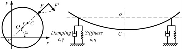
As shown in Fig. 1, the rotor system is considered as a single-span rotor supported by force $F$ , which can be divided into stiffness force and damping force. Noticing that, the force $F'$ , which is perpendicular to $F$ and caused by sealing force, is not considered in this paper, so that we can formulate this model with single DOF instead of the traditional crossing two DOF. By introducing nonlinear Hooke’s law and nonlinear damping force, we can construct nonlinear analytical model with single DOF.

Fig. 1Dynamic analysis for a rotor

2.1. Nonlinear stiffness

From the perspective of elastic theory, based on the hypothesis of small perturbation and deformation, traditional model for representing flexible rotor behaviors can be generally satisfied with Hooke’s law. However, under the circumstances of large perturbation or deformation, the elastic potential energy of one-dimensional system [14] can be expressed as:

1

U (x) = \frac{1}{2} k x^{2} + \frac{1}{3} ξ x^{3} + \frac{1}{4} η x^{4} + \dots .

For engineering practice, the potential energy of many structures can be considered as symmetry [15]. Thus, the even order terms of Eq. (1) are retained:

2

U (x) = \frac{1}{2} k x^{2} + \frac{1}{4} η x^{4} .

The stiffness force $f_{k}$ , namely the elastic force, is expressed as:

3

f_{k} = - \frac{d U}{d x} = - k x - η x^{3} .

where $k$ is the coefficient of linear elastic deformation, namely stiffness, $η$ is the coefficient of nonlinear elastic deformation. If $η =$ 0, Eq. (3) satisfies the linear Hooke’s law, namely linear spring characteristics. If $η >$ 0, $f_{k}$ increases along with deformation increasing, namely hard spring characteristics. On the contrary, if $η <$ 0, $f_{k}$ decreases along with deformation increasing, namely soft spring characteristics [16].

2.2. Nonlinear damping

Generally, the damping dissipation process of non-conservative system [17] can be given as:

4

m \ddot{x} + q (\dot{x}) + k x = 0 .

Thus, the damping force is described as a generalized form:

5

q (\dot{x}) = - c {|\dot{x}|}^{n - 1} \dot{x}, (n = 0,1, 2, . . .) .

If $n =$ 0, Eq. (5) represents dry friction force. If $n =$ 1, Eq. (5) represents linear viscous damping force, which is applied to low-speed movement in fluid. If $n =$ 2, Eq. (5) represents nonlinear viscous damping force, which is applied to high-speed movement [18]. Thus, the damping force $f_{c}$ is expressed as:

6

f_{c} = - c \dot{x} - γ {\dot{x}}^{2},

where $c$ represents linear damping, $γ$ is the coefficient of nonlinear damping.

2.3. Analytical model

Considering the single-span single-disc rotor system shown in Fig. 1, the parameters are as follows, $m$ for disc mass, $r$ for eccentricity, $Ω$ for rotational frequency. And shaft mass is ignored, counterclockwise is positive. For general liquid or gas bearing, there is interaction of support and whirl, due to wedge flow characteristics. In this context, we consider only bearing supporting effect, so that based on Newton’s second law, equation of motion in the $x$ -axis direction can be described as:

7

m \frac{d^{2} x_{C}}{d t^{2}} = - k x - η x^{3} - c \dot{x} - γ {\dot{x}}^{2},

where:

8

x_{C} = x + r c o s Ω t .

For briefness and clarity, some substitutions are given as:

9

\begin{array}{l} μ = \frac{c}{2 m}, & ε β_{0}^{2} = \frac{η}{m}, & ω_{0}^{2} = \frac{k}{m}, & ε α_{0}^{2} = \frac{γ}{m} \end{array},

where $μ$ is linear damping coefficient, $ω_{0}$ is natural frequency, $β_{0}$ is nonlinear stiffness amplification coefficient, $α_{0}$ is nonlinear damping amplification coefficient, $ε$ is the nonlinear scale factor which denotes the impact of nonlinear responses of rotor system.

Then, the analytical model for nonlinear vibration of flexible rotor system can be written as:

10

\ddot{x} + 2 μ \dot{x} + ε α_{0}^{2} {\dot{x}}^{2} + ω_{0}^{2} x + ε β_{0}^{2} x^{3} = Ω^{2} r c o s Ω t .

Noticing that, Eq. (10) has a similar form with Duffing equation [19], in which $x^{3}$ term is used to describe nonlinear elastic restoring force. Numerous researches show that the response characteristics of complex rotor system is consistent with the analysis of single DOF Duffing equation in many respects, such as period-doubling bifurcation, Hopf bifurcation, period-3 bifurcation, enter/exit chaos phenomenon [20].

This analytical model Eq. (10) deals with centrifugal force generated by unbalanced mass, essentially not as the same as Muszynska model, which aims to deal with the clearance force caused by sealing fluid (that is why the negative sign exists as a reaction force in Eq. (11), which is different from that in Eq. (10) as an action force). If the nonlinear scale factor $ε$ is very small, the nonlinear terms can be neglected. Then considering linear interaction of stiffness and damping, i.e., cross stiffness and cross damping force, Eq. (10) can be transformed into Muszynska model [11]:

11

- [\begin{array}{l} F_{x} \\ F_{y} \end{array}] = [\begin{matrix} k - m_{f} τ^{2} ω^{2} & τ ω c \\ - τ ω c & k - m_{f} τ^{2} ω^{2} \end{matrix}] [\begin{array}{l} x \\ y \end{array}] + [\begin{matrix} c & 2 τ ω m_{f} \\ - 2 τ ω m_{f} & c \end{matrix}] [\begin{array}{l} \dot{x} \\ \dot{y} \end{array}] + [\begin{matrix} m_{f} & 0 \\ 0 & m_{f} \end{matrix}] [\begin{array}{l} \ddot{x} \\ \ddot{y} \end{array}] .

On this basis, if ignore inertial force, and substitute coefficients for simple letters, Eq. (11) can be simplified as Alford model [6]:

12

- [\begin{array}{l} F_{x} \\ F_{y} \end{array}] = [\begin{matrix} k_{1} & k_{2} \\ - k_{2} & k_{1} \end{matrix}] [\begin{array}{l} x \\ y \end{array}] + [\begin{matrix} c_{1} & c_{2} \\ - c_{2} & c_{1} \end{matrix}] [\begin{array}{l} \dot{x} \\ \dot{y} \end{array}] .

Apparently, if the cross damping force is not considered, Eq. (11) can be simplified as Ravikovich model [12]:

13

m \ddot{x} + 2 c \dot{x} + 2 k_{x x} x + 2 k_{x y} y = - m r ω^{2} s i n ω t,

m \ddot{y} + 2 c \dot{y} + 2 k_{y y} y + 2 k_{y x} x = - m r ω^{2} c o s ω t,

where $F$ is excitation force, $k$ is stiffness, $c$ is damping, $τ$ is fluid circumferential average velocity ratio, $m_{f}$ is inertial mass, $ω$ is rotational speed, $m$ is mass, $r$ is eccentricity, in Eq. (11-13).

Fig. 2Schematic of linear response and nonlinear response

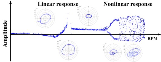
Apparently, these models mentioned above used cross terms to describe nonlinear characteristics indirectly. In this paper, the analytical model introduces nonlinear stiffness force and nonlinear damping force instead of cross terms, i.e., Eq. (3) and Eq. (6), to directly describe the nonlinear effects with clear physical significance, and then to do further research on the interaction of linear and nonlinear forces, and the mechanism of nonlinear dynamic responses under the conditions of large displacement and high speed. Fig. 2 shows the linear and nonlinear response characteristics in frequency domain.

3. Analytical solutions and analysis

3.1. Free vibration mode

Multi-scale method can calculate both of the steady-state response and the transient-state response. In order to represent different time scales, $T_{n}$ is introduced and defined as:

14

T_{n} = ε^{n} t, (n = 0,1, 2, . . .) .

Then, a nonlinear response can be written as a function of various time scales:

15

x = \sum_{n = 0}^{m} ε^{n} x_{n} (T_{0}, T_{1}, T_{2}, . . ., T_{m}),

where $n$ depends on the calculation accuracy.

When an external excitation does not exist, the free vibration mode of the analytical model can be expressed as:

16

\ddot{x} + 2 μ \dot{x} + ε α_{0}^{2} {\dot{x}}^{2} + ω_{0}^{2} x + ε β_{0}^{2} x^{3} = 0 .

Based on multi-scale method, we suppose:

17

x = x_{0} (T_{0}, T_{1}) + ε x_{1} (T_{0}, T_{1}),

where:

18

T_{0} = t, T_{1} = ε t .

Thus:

19

\dot{x} = \frac{\partial x_{0}}{\partial T_{0}} + ε \frac{\partial x_{0}}{\partial T_{1}} + ε \frac{\partial x_{1}}{\partial T_{0}} + ε^{2} \frac{\partial x_{1}}{\partial T_{1}},

\ddot{x} = \frac{\partial^{2} x_{0}}{\partial {T_{0}}^{2}} + 2 ε \frac{\partial^{2} x_{0}}{\partial T_{0} \partial T_{1}} + ε^{2} \frac{\partial^{2} x_{0}}{\partial {T_{1}}^{2}} + ε \frac{\partial^{2} x_{1}}{\partial {T_{0}}^{2}} + 2 ε^{2} \frac{\partial^{2} x_{1}}{\partial T_{0} \partial T_{1}} + ε^{3} \frac{\partial^{2} x_{1}}{\partial {T_{1}}^{2}} .

Then, according to the power orders of $ε$ , there are:

20

ε^{0} : D_{0}^{2} x_{0} + 2 μ D_{0} x_{0} + ω_{0}^{2} x_{0} = 0,

21

ε^{1} : D_{0}^{2} x_{1} + 2 μ D_{0} x_{1} + ω_{0}^{2} x_{1} = - 2 D_{0} D_{1} x_{0} - 2 μ D_{1} x_{0} - α_{0}^{2} {(D_{0} x_{0})}^{2} - β_{0}^{2} x_{0}^{3},

where $D_{n}$ ( $n =$ 0, 1) is the partial differential operator. The solution of Eq. (20) is:

22

x_{0} = C (T_{1}) e^{r_{1} T_{0}} + \bar{C} (T_{1}) e^{{\bar{r}}_{1} T_{0}}, r_{1} = - μ + j \sqrt{ω_{0}^{2} - μ^{2}},

where $C$ is an unknown complex function, the overline represents the conjugate function. Take Eq. (22) into Eq. (21), we have:

23

D_{0}^{2} x_{1} + 2 μ D_{0} x_{1} + ω_{0}^{2} x_{1} = - [2 D_{1} C (r_{1} + μ) + 3 β_{0}^{2} C^{2} \bar{C} e^{- 2 μ T_{0}}] e^{r_{1} T_{0}}

- α_{0}^{2} C \bar{C} r_{1} {\bar{r}}_{1} e^{- 2 μ T_{0}} - α_{0}^{2} C^{2} r_{1}^{2} e^{2 r_{1} T_{0}} - β_{0}^{2} C^{3} e^{3 r_{1} T_{0}} + c c,

where $c c$ represents the conjugate functions of each term before. The coefficient of first term $e^{r_{1} T_{0}}$ must be zero to avoid duration term. At any point without acceleration, $T_{0} = 0$ , so $e^{- 2 μ T_{0}} = 1$ . There is:

24

2 D_{1} C (μ + r_{1}) + 3 β_{0}^{2} C^{2} \bar{C} = 0 .

Assuming:

25

C = \frac{1}{2} a e^{j φ},

where $a$ and $φ$ are the functions of $T_{1}$ . According to the real part and the imaginary part respectively, $C$ can be obtained:

26

C = \frac{1}{2} a_{0} e^{j \frac{3 β_{0}^{2} a_{0}^{2}}{8 \sqrt{ω_{0}^{2} - μ^{2}}} T_{1} + j φ_{0}},

where $a_{0}$ , $φ_{0}$ are the integration constants. Take Eq. (26) and Eq. (22) into Eq. (23), $x_{1}$ can be solved, then the solution $x$ is:

27

x = \frac{1}{2} a_{0} e^{- μ t + j \sqrt{ω_{0}^{2} - μ^{2}} t + j \frac{3 ε β_{0}^{2} a_{0}^{2}}{8 \sqrt{ω_{0}^{2} - μ^{2}}} t + j φ_{0}} - \frac{1}{4} ε α_{0}^{2} a_{0}^{2} e^{- 2 μ t}

+ \frac{ε α_{0}^{2} a_{0}^{2} (2 μ^{2} - ω_{0}^{2} - 2 j μ \sqrt{ω_{0}^{2} - μ^{2}})}{4 (- 4 μ^{2} + 3 ω_{0}^{2} + 4 j μ \sqrt{ω_{0}^{2} - μ^{2}})} e^{- 2 μ t + 2 j \sqrt{ω_{0}^{2} - μ^{2}} t + j \frac{3 ε β_{0}^{2} a_{0}^{2}}{4 \sqrt{ω_{0}^{2} - μ^{2}}} t + 2 j φ_{0}}

+ \frac{ε β_{0}^{2} a_{0}^{3}}{32 (- 3 μ^{2} + 2 ω_{0}^{2} + 3 j μ \sqrt{ω_{0}^{2} - μ^{2}})} e^{- 3 μ t + 3 j \sqrt{ω_{0}^{2} - μ^{2}} t + j \frac{9 ε β_{0}^{2} a_{0}^{2}}{8 \sqrt{ω_{0}^{2} - μ^{2}}} t + 3 j φ_{0}} + c c .

Thus, the natural frequency is:

28

ω = \sqrt{ω_{0}^{2} - μ^{2}} + \frac{3 ε β_{0}^{2} a_{0}^{2}}{8 \sqrt{ω_{0}^{2} - μ^{2}}} = \sqrt{ω_{0}^{2} - μ^{2}} + \frac{3 a_{0}^{2}}{8 m \sqrt{ω_{0}^{2} - μ^{2}}} η,

where the first term on the right side is linear natural frequency and the second is nonlinear natural frequency. Obviously, $ω_{0}$ , $μ$ , $β_{0}$ and $η$ have an impact on the natural frequency but $α_{0}$ , $γ$ does not.

3.2. Forced vibration mode

When the external excitation exists, for instance centrifugal force caused by unbalanced mass of the rotor, the forced vibration mode of analytical model can be expressed as:

29

\ddot{x} + 2 μ \dot{x} + ε α_{0}^{2} {\dot{x}}^{2} + ω_{0}^{2} x + ε β_{0}^{2} x^{3} = Ω^{2} r c o s Ω t .

Similarly, using multi-scale method, according to the power orders of $ε$ , there are:

30

ε^{0} : D_{0}^{2} x_{0} + 2 μ D_{0} x_{0} + ω_{0}^{2} x_{0} = \frac{1}{2} Ω^{2} r (e^{j Ω T_{0}} + e^{- j Ω T_{0}}),

31

ε^{1} : D_{0}^{2} x_{1} + 2 μ D_{0} x_{1} + ω_{0}^{2} x_{1} = - 2 D_{0} D_{1} x_{0} - 2 μ D_{1} x_{0} - α_{0}^{2} {(D_{0} x_{0})}^{2} - β_{0}^{2} x_{0}^{3} .

The solution of Eq. (30) is:

32

x_{0} = C (T_{1}) e^{r_{1} T_{0}} + \bar{C} (T_{1}) e^{{\bar{r}}_{1} T_{0}} + Q e^{j Ω T_{0}} + \bar{Q} e^{- j Ω T_{0}},

r_{1} = - μ + j \sqrt{ω_{0}^{2} - μ^{2}}, Q = \frac{1}{2} \frac{Ω^{2} r}{ω_{0}^{2} - Ω^{2} + 2 j μ Ω},

where $C$ is an unknown complex function, the overline represents the conjugate function. Take Eq. (32) into Eq. (31), we have:

33

D_{0}^{2} x_{1} + 2 μ D_{0} x_{1} + ω_{0}^{2} x_{1} = - [2 D_{1} C (r_{1} + μ) + 6 β_{0}^{2} C Q Q + 3 β_{0}^{2} C^{2} \bar{C} e^{- 2 μ T_{0}}] e^{r_{1} T_{0}}

- α_{0}^{2} Q \bar{Q} Ω^{2} - α_{0}^{2} C \bar{C} r_{1} {\bar{r}}_{1} e^{- 2 μ T_{0}} - 3 β_{0}^{2} Q^{2} \bar{Q} e^{j Ω T_{0}} + α_{0}^{2} Q^{2} Ω^{2} e^{2 j Ω T_{0}} - β_{0}^{2} Q^{3} e^{3 j Ω T_{0}}

- 2 j α_{0}^{2} C r_{1} Q Ω e^{r_{1} T_{0} + j Ω T_{0}} + 2 j α_{0}^{2} C r_{1} \bar{Q} Ω e^{r_{1} T_{0} - j Ω T_{0}} - 6 β_{0}^{2} C \bar{C} Q e^{- 2 μ T_{0} + j Ω T_{0}}

- 3 β_{0}^{2} C^{2} Q e^{2 r_{1} T_{0} + j Ω T_{0}} - 3 β_{0}^{2} C^{2} \bar{Q} e^{2 r_{1} T_{0} - j Ω T_{0}} - 3 β_{0}^{2} C Q^{2} e^{r_{1} T_{0} + 2 j Ω T_{0}}

- 3 β_{0}^{2} C {\bar{Q}}^{2} e^{r_{1} T_{0} - 2 j Ω T_{0}} - α_{0}^{2} C^{2} r_{1}^{2} e^{2 r_{1} T_{0}} - β_{0}^{2} C^{3} e^{3 r_{1} T_{0}} + c c .

Similarly, to avoid duration term, the coefficient of first term $e^{r_{1} T_{0}}$ must be zero. At any point without acceleration, $T_{0} = 0$ , so $e^{- 2 μ T_{0}} = 1$ . There is:

34

2 D_{1} C (r_{1} + μ) + 6 β_{0}^{2} C Q \bar{Q} + 3 β_{0}^{2} C^{2} \bar{C} = 0 .

Take Eq. (25) into Eq. (34), according to the real part and the imaginary part respectively, $C$ can be obtained.

35

C = \frac{1}{2} a_{0} e^{j \frac{\frac{6 β_{0}^{2} Ω^{4} r^{2}}{{(ω_{0}^{2} - Ω^{2})}^{2} + 4 μ^{2} Ω^{2}} + 3 β_{0}^{2} a_{0}^{2}}{8 \sqrt{ω_{0}^{2} - μ^{2}}} T_{1} + j φ_{0}},

where $a_{0}$ , $φ_{0}$ are the integration constants. Take Eq. (35) and Eq. (32) into Eq. (33), $x_{1}$ can be solved, then the solution $x$ is:

x = \frac{1}{2} a_{0} \exp (- μ t + j \sqrt{ω_{0}^{2} - μ^{2}} t + j \frac{\frac{6 ε β_{0}^{2} Ω^{4} r^{2}}{{(ω_{0}^{2} - Ω^{2})}^{2} + 4 μ^{2} Ω^{2}} + 3 ε β_{0}^{2} a_{0}^{2}}{8 \sqrt{ω_{0}^{2} - μ^{2}}} t + j φ_{0})

+ \frac{1}{2} \frac{Ω^{2} r}{ω_{0}^{2} - Ω^{2} + 2 j μ Ω} e^{j Ω t} - \frac{1}{4} ε α_{0}^{2} a_{0}^{2} e^{- 2 μ t}

- \frac{ε α_{0}^{2} Ω^{6} r^{2}}{4 ω_{0}^{2} [{(ω_{0}^{2} - Ω^{2})}^{2} + 4 μ^{2} Ω^{2}]} - \frac{3 ε β_{0}^{2} Ω^{6} r^{3}}{8 {(ω_{0}^{2} - Ω^{2} + 2 j μ Ω)}^{3} (ω_{0}^{2} - Ω^{2} - 2 j μ Ω)} e^{j Ω t}

+ \frac{ε α_{0}^{2} Ω^{6} r^{2}}{4 (ω_{0}^{2} - 4 Ω^{2} + 4 j μ Ω) {(ω_{0}^{2} - Ω^{2} + 2 j μ Ω)}^{2}} e^{2 j Ω t} - \frac{3 ε β_{0}^{2} a_{0}^{2} Ω^{2} r}{4 [{(ω_{0}^{2} - Ω^{2})}^{2} + 4 μ^{2} Ω^{2}]} e^{- 2 μ t + j Ω t}

- \frac{ε β_{0}^{2} Ω^{6} r^{3}}{8 (ω_{0}^{2} - 9 Ω^{2} + 6 j μ Ω) {(ω_{0}^{2} - Ω^{2} + 2 j μ Ω)}^{3}} e^{3 j Ω t} - \frac{ε α_{0}^{2} a_{0} Ω^{2} r (j μ + \sqrt{ω_{0}^{2} - μ^{2}})}{2 (2 \sqrt{ω_{0}^{2} - μ^{2}} + Ω) (ω_{0}^{2} - Ω^{2} + 2 j μ Ω)}

\times \exp (- μ t + j \sqrt{ω_{0}^{2} - μ^{2}} t + j Ω t + j \frac{\frac{6 ε β_{0}^{2} Ω^{4} r^{2}}{{(ω_{0}^{2} - Ω^{2})}^{2} + 4 μ^{2} Ω^{2}} + 3 ε β_{0}^{2} a_{0}^{2}}{8 \sqrt{ω_{0}^{2} - μ^{2}}} t + j φ_{0})

- \frac{ε α_{0}^{2} a_{0} Ω^{2} r (j μ + \sqrt{ω_{0}^{2} - μ^{2}})}{2 (2 \sqrt{ω_{0}^{2} - μ^{2}} - Ω) (ω_{0}^{2} - Ω^{2} - 2 j μ Ω)}

\times \exp (- μ t + j \sqrt{ω_{0}^{2} - μ^{2}} t - j Ω t + j \frac{\frac{6 ε β_{0}^{2} Ω^{4} r^{2}}{{(ω_{0}^{2} - Ω^{2})}^{2} + 4 μ^{2} Ω^{2}} + 3 ε β_{0}^{2} a_{0}^{2}}{8 \sqrt{ω_{0}^{2} - μ^{2}}} t + j φ_{0})

+ \frac{3 ε β_{0}^{2} a_{0}^{2} Ω^{2} r e x p (- 2 μ t + 2 j \sqrt{ω_{0}^{2} - μ^{2}} t + j Ω t + j \frac{\frac{6 ε β_{0}^{2} Ω^{4} r^{2}}{{(ω_{0}^{2} - Ω^{2})}^{2} + 4 μ^{2} Ω^{2}} + 3 ε β_{0}^{2} a_{0}^{2}}{4 \sqrt{ω_{0}^{2} - μ^{2}}} t + 2 j φ_{0})}{8 (- 4 μ^{2} + 3 ω_{0}^{2} + 4 j μ \sqrt{ω_{0}^{2} - μ^{2}} + Ω^{2} + 2 j μ Ω + 4 Ω \sqrt{ω_{0}^{2} - μ^{2}}) (ω_{0}^{2} - Ω^{2} + 2 j μ Ω)}

+ \frac{3 ε β_{0}^{2} a_{0}^{2} Ω^{2} r e x p (- 2 μ t + 2 j \sqrt{ω_{0}^{2} - μ^{2}} t - j Ω t + j \frac{\frac{6 ε β_{0}^{2} Ω^{4} r^{2}}{{(ω_{0}^{2} - Ω^{2})}^{2} + 4 μ^{2} Ω^{2}} + 3 ε β_{0}^{2} a_{0}^{2}}{4 \sqrt{ω_{0}^{2} - μ^{2}}} t + 2 j φ_{0})}{8 (- 4 μ^{2} + 3 ω_{0}^{2} + 4 j μ \sqrt{ω_{0}^{2} - μ^{2}} + Ω^{2} - 2 j μ Ω - 4 Ω \sqrt{ω_{0}^{2} - μ^{2}}) (ω_{0}^{2} - Ω^{2} - 2 j μ Ω)}

+ \frac{3 ε β_{0}^{2} a_{0} Ω^{3} r^{2}}{32 (\sqrt{ω_{0}^{2} - μ^{2}} + Ω) {(ω_{0}^{2} - Ω^{2} + 2 j μ Ω)}^{2}}

\times \exp (- μ t + j \sqrt{ω_{0}^{2} - μ^{2}} t + 2 j Ω t + j \frac{\frac{6 ε β_{0}^{2} Ω^{4} r^{2}}{{(ω_{0}^{2} - Ω^{2})}^{2} + 4 μ^{2} Ω^{2}} + 3 ε β_{0}^{2} a_{0}^{2}}{8 \sqrt{ω_{0}^{2} - μ^{2}}} t + j φ_{0})

+ \frac{3 ε β_{0}^{2} a_{0} Ω^{3} r^{2}}{32 (- \sqrt{ω_{0}^{2} - μ^{2}} + Ω) {(ω_{0}^{2} - Ω^{2} - 2 j μ Ω)}^{2}}

\times \exp (- μ t + j \sqrt{ω_{0}^{2} - μ^{2}} t - 2 j Ω t + j \frac{\frac{6 ε β_{0}^{2} Ω^{4} r^{2}}{{(ω_{0}^{2} - Ω^{2})}^{2} + 4 μ^{2} Ω^{2}} + 3 ε β_{0}^{2} a_{0}^{2}}{8 \sqrt{ω_{0}^{2} - μ^{2}}} t + j φ_{0})

+ \frac{ε α_{0}^{2} a_{0}^{2} (2 μ^{2} - ω_{0}^{2} - 2 j μ \sqrt{ω_{0}^{2} - μ^{2}})}{4 (- 4 μ^{2} + 3 ω_{0}^{2} + 4 j μ \sqrt{ω_{0}^{2} - μ^{2}})}

\times \exp (- 2 μ t + 2 j \sqrt{ω_{0}^{2} - μ^{2}} t + j \frac{\frac{6 ε β_{0}^{2} Ω^{4} r^{2}}{{(ω_{0}^{2} - Ω^{2})}^{2} + 4 μ^{2} Ω^{2}} + 3 ε β_{0}^{2} a_{0}^{2}}{4 \sqrt{ω_{0}^{2} - μ^{2}}} t + 2 j φ_{0})

+ \frac{ε β_{0}^{2} a_{0}^{3}}{32 (- 3 μ^{2} + 2 ω_{0}^{2} + 3 j μ \sqrt{ω_{0}^{2} - μ^{2}})}

\times \exp (- 3 μ t + 3 j \sqrt{ω_{0}^{2} - μ^{2}} t + j \frac{\frac{18 ε β_{0}^{2} Ω^{4} r^{2}}{{(ω_{0}^{2} - Ω^{2})}^{2} + 4 μ^{2} Ω^{2}} + 9 ε β_{0}^{2} a_{0}^{2}}{8 \sqrt{ω_{0}^{2} - μ^{2}}} t + 3 j φ_{0}) + c c .

To do further simplification, the solution $x$ is:

36

x = A_{0} c o s (Ω t + θ_{0}) + A_{1} c o s (Ω t + θ_{1}) + A_{2} c o s (2 Ω t + θ_{2}) + A_{3} c o s (3 Ω t + θ_{3}) + A_{4}

+ a_{0} e^{- μ t} c o s (φ t + φ_{0}) + A_{01} e^{- 2 μ t} c o s Ω t + A_{40} e^{- 2 μ t}

+ A_{11} e^{- μ t} c o s ((φ + Ω) t + θ_{11}) + A_{11'} e^{- μ t} c o s ((φ - Ω) t + θ_{11'})

+ A_{21} e^{- 2 μ t} c o s ((2 φ + Ω) t + θ_{21}) + A_{21'} e^{- 2 μ t} c o s ((2 φ - Ω) t + θ_{21'})

+ A_{12} e^{- μ t} c o s ((φ + 2 Ω) t + θ_{12}) + A_{12'} e^{- μ t} c o s ((φ - 2 Ω) t + θ_{12'})

+ A_{20} e^{- 2 μ t} c o s (2 φ t + θ_{20}) + A_{30} e^{- 3 μ t} c o s (3 φ t + θ_{30}),

where:

37

A_{0} = \frac{r}{\sqrt{{(λ^{2} - 1)}^{2} + δ^{2}}}, A_{1} = - \frac{3 ε β_{0}^{2}}{4 Ω^{2} r} A_{0}^{4}, A_{2} = \frac{ε α_{0}^{2}}{2 \sqrt{{(λ^{2} - 4)}^{2} + 4 δ^{2}}} A_{0}^{2},

A_{3} = - \frac{ε β_{0}^{2}}{4 Ω^{2} \sqrt{{(λ^{2} - 9)}^{2} + 9 δ^{2}}} A_{0}^{3}, A_{4} = - \frac{ε α_{0}^{2}}{2 λ^{2}} A_{0}^{2}, A_{01} = - \frac{3 ε β_{0}^{2} a_{0}^{2}}{2 Ω^{2} r} A_{0}^{2},

A_{11} = - \frac{ε α_{0}^{2} a_{0} λ}{\sqrt{4 λ^{2} - δ^{2}} + 1} A_{0}, A_{12} = \frac{3 ε β_{0}^{2} a_{0}}{8 Ω^{2} (\sqrt{4 λ^{2} - δ^{2}} + 2)} A_{0}^{2},

A_{21} = \frac{3 ε β_{0}^{2} a_{0}^{2}}{4 Ω^{2} \sqrt{{(3 λ^{2} + 1 - δ^{2} + 2 \sqrt{4 λ^{2} - δ^{2}})}^{2} + {(δ \sqrt{4 λ^{2} - δ^{2}} + δ)}^{2}}} A_{0},

A_{20} = \frac{ε α_{0}^{2} a_{0}^{2} \sqrt{{(- 2 λ^{2} + δ^{2})}^{2} + δ^{2} (4 λ^{2} - δ^{2})}}{4 \sqrt{{(3 λ^{2} - δ^{2})}^{2} + δ^{2} (4 λ^{2} - δ^{2})}},

A_{30} = \frac{ε β_{0}^{2} a_{0}^{3}}{4 Ω^{2} \sqrt{{(8 λ^{2} - 3 δ^{2})}^{2} + 9 δ^{2} (4 λ^{2} - δ^{2})}},

A_{40} = - \frac{1}{2} ε α_{0}^{2} a_{0}^{2}, θ_{11} = a r c t g \frac{δ}{\sqrt{4 λ^{2} - δ^{2}}} + θ_{0} + φ_{0}, A_{11^{'}} = - \frac{ε α_{0}^{2} a_{0} λ}{\sqrt{4 λ^{2} - δ^{2}} - 1} A_{0},

A_{21^{'}} = \frac{3 ε β_{0}^{2} a_{0}^{2}}{4 Ω^{2} \sqrt{{(3 λ^{2} + 1 - δ^{2} - 2 \sqrt{4 λ^{2} - δ^{2}})}^{2} + {(δ \sqrt{4 λ^{2} - δ^{2}} - δ)}^{2}}} A_{0},

A_{12^{'}} = \frac{3 ε β_{0}^{2} a_{0}}{8 Ω^{2} (- \sqrt{4 λ^{2} - δ^{2}} + 2)} A_{0}^{2},

λ = \frac{ω_{0}}{Ω}, δ = \frac{2 μ}{Ω}, φ = \frac{1}{2} Ω \sqrt{4 λ^{2} - δ^{2}} + \frac{3 ε β_{0}^{2} (2 A_{0}^{2} + a_{0}^{2})}{4 Ω \sqrt{4 λ^{2} - δ^{2}}},

θ_{0} = - a r c t g \frac{δ}{λ^{2} - 1}, θ_{1} = 2 θ_{0}, θ_{2} = - a r c t g \frac{2 δ}{λ^{2} - 4} + 2 θ_{0},

θ_{3} = - a r c t g \frac{3 δ}{λ^{2} - 9} + 3 θ_{0}, θ_{21} = - a r c t g \frac{δ \sqrt{4 λ^{2} - δ^{2}} + δ}{3 λ^{2} + 1 - δ^{2} + 2 \sqrt{4 λ^{2} - δ^{2}}} + θ_{0} + 2 φ_{0},

{θ_{12} = 2 θ_{0} + φ_{0}, θ}_{20} = - a r c t g \frac{δ \sqrt{4 λ^{2} - δ^{2}}}{- 2 λ^{2} + δ^{2}} - a r c t g \frac{δ \sqrt{4 λ^{2} - δ^{2}}}{3 λ^{2} - δ^{2}} + 2 φ_{0},

θ_{30} = - a r c t g \frac{3 δ \sqrt{4 λ^{2} - δ^{2}}}{8 λ^{2} - 3 δ^{2}} + 3 φ_{0}, θ_{11^{'}} = a r c t g \frac{δ}{\sqrt{4 λ^{2} - δ^{2}}} - θ_{0} + φ_{0},

θ_{21^{'}} = - a r c t g \frac{δ \sqrt{4 λ^{2} - δ^{2}} - δ}{3 λ^{2} + 1 - δ^{2} - 2 \sqrt{4 λ^{2} - δ^{2}}} - θ_{0} + 2 φ_{0}, θ_{12^{'}} = - 2 θ_{0} + φ_{0},

where $λ$ is rotational speed ratio, $δ$ is damping rotational speed ratio, $A_{i}$ represents amplitude, $θ_{i}$ represents phase. Eq. (36) is the complete expression of solution $x$ , including steady-state and transient-state. When the time $t$ is large enough, $e^{- μ t}$ decays to 0 rapidly, so the transient-state solution vanishes. Then Eq. (36) degenerates into the steady-state solution as follows:

38

x = A_{0} c o s (Ω t + θ_{0}) + A_{1} c o s (Ω t + θ_{1}) + A_{2} c o s (2 Ω t + θ_{2}) + A_{3} c o s (3 Ω t + θ_{3}) + A_{4} .

Notice that, when rotational speed changes with time, Eq. (36) and Eq. (38) are not satisfied with the basic assumption of Fourier transform, which requires amplitude and phase to be time-invariant. Therefore, short-time Fourier transform (STFT) can be used to obtain an approximate frequency-domain solution.

If nonlinear scale factor $ε$ equals zero, $A_{1} = A_{2} = A_{3} = A_{4} = 0$ , then Eq. (38) degenerates into the traditional linear response $A_{0} c o s (Ω t + θ_{0})$ . The mechanism of nonlinear scale factor $ε$ is fully clarified that the magnitude of $ε$ reflects the degree of nonlinear influence, furthermore, it is also verifies the rationality and validity of the analytical model.

3.3. Frequency response equation (FRE)

Generally, under an external excitation caused by an unbalanced force, the linear response belongs to single fundamental frequency response, but the nonlinear response may include a series of harmonic responses. For general engineering applications, working frequency FRE is often used to analyze instability problems. Considering the first two terms on the right side of Eq. (38), according to wave superposition principle, there is:

39

A_{0} c o s (Ω t + θ_{0}) + A_{1} c o s (Ω t + θ_{1}) = A_{a} c o s (Ω t + θ_{a}),

where:

40

A_{a}^{2} = A_{0}^{2} + A_{1}^{2} + 2 A_{0} A_{1} c o s (θ_{0} - θ_{1}) .

Assuming $A_{a} = a$ , substituting $A_{1}$ and $θ_{1}$ of Eq. (37), we have:

41

a^{2} = A_{0}^{2} + \frac{9 ε^{2} β_{0}^{4}}{16 Ω^{4} r^{2}} A_{0}^{8} - \frac{3 ε β_{0}^{2}}{2 Ω^{2} r} A_{0}^{5} c o s θ_{0} .

To simplify:

42

- \frac{9}{16} ε^{2} β_{0}^{4} A_{0}^{6} + \frac{3}{2} ε β_{0}^{2} (ω_{0}^{2} - Ω^{2}) A_{0}^{4} + [{(ω_{0}^{2} - Ω^{2})}^{2} + 4 μ^{2} Ω^{2}] a^{2} = Ω^{4} r^{2} .

If $A_{0}^{2} = a^{2} - \frac{9 ε^{2} β_{0}^{4}}{16 Ω^{4} r^{2}} A_{0}^{8} + \frac{3 ε β_{0}^{2}}{2 Ω^{2} r} A_{0}^{5} c o s θ_{0} \approx a^{2}$ , the nonlinear FRE can be derived as:

43

- \frac{9}{16} ε^{2} β_{0}^{4} a^{6} + \frac{3}{2} ε β_{0}^{2} (ω_{0}^{2} - Ω^{2}) a^{4} + [{(ω_{0}^{2} - Ω^{2})}^{2} + 4 μ^{2} Ω^{2}] a^{2} = Ω^{4} r^{2} .

Thus, it can help to explain why the working frequency FRE cannot reflect the nonlinear characteristics accurately, or even analyze some nonlinear problems efficiently in engineering applications. The comparison between experimental result and analytical solution is given below.

4. Experimental Facility and procedure

Table 1 shows the main parameters of the test rig.

Table 1Main parameters of the test rig

Relevant parameters	Values
Rotor material	40 Cr
Rotor mass	10.36 kg
Rotor length	698 mm
Bearing inner diameter	50 mm
Radial clearance	0.02 mm
Clearance ratio	0.0016
Shaft diameter	50 mm
Bearing length	60 mm
Thrust disc diameter	90 mm
Bearing span	525 mm

Fig. 3 [21] shows the schematic of the gas-bearing rotor system test rig, gas supply system, as well as the vibration signal acquisition and analysis system. The test rig has a single-stage radial turbine coaxial with a shaft driven by high-pressure air and maximum speed of 1.2×10⁵ rpm. A screw-type air compressor provides high-pressure air with maximum pressure of 1.2 MPa and maximum mass flow of 3.90 kg/s. The airflow into the bearings is controlled by stabilizing valves and air regulators. A K-type thermocouple monitors the temperature of the supply gas. A calibrated mass flowmeter measures the mass flow rate into each bearing with an uncertainty of 0.195 kg/s. The regulators control the air pressure in proportion to the rotational speed in the speed-up process.

Fig. 3Layout of the rotor system test rig and gas supply system: 1) air compressor, 2) gas tank, 3) filter, 4) dryer, 5) pressure gauge, 6) thermometer, 7) flowmeter, 8) pressure stabilizing valve, 9) electro-pneumatic air regulator, 10) safety shut-off valve, 11) computer, 12) data acquisition instrument, 13) eddy current sensor

Layout of the rotor system test rig and gas supply system: 1) air compressor, 2) gas tank, 3) filter, 4) dryer, 5) pressure gauge, 6) thermometer, 7) flowmeter, 8) pressure stabilizing valve, 9) electro-pneumatic air regulator, 10) safety shut-off valve, 11) computer, 12) data acquisition instrument, 13) eddy current sensor

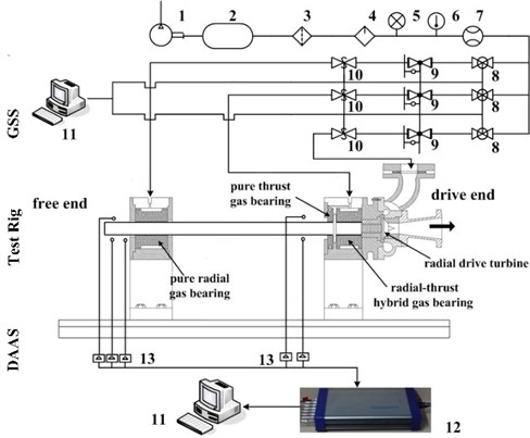
Two pairs of eddy current displacement sensors, which are orthogonally positioned near test bearings, are used to measure the rotor lateral vibration amplitudes along the $X$ -horizontal and $Y$ -vertical axis. An eddy current key phase sensor mounted at the free end of the rotor is used to measure the phase signal. The displacement range is of 1 mm. The linearity is of 10.4 V/mm, and the frequency range is of 0-10 kHz. The sensor signals through filters and amplifiers are input to the acquisition and analysis system for real-time monitoring, storage, and analysis [22].

5. Results and discussion

The theoretical calculation is accomplished with the parameter assignment as follows, $m =$ 1 kg, $k =$ 1×10⁴ N/m, $c =$ 20 Ns/m, $r =$ 1×10^-5 m, $η =$ 2.5×10¹² N/m³, $γ =$ 8×10⁴ Ns²/m², thus $ω_{0} =$ 100 rad/s, $μ =$ 10 rad/s. Using Matlab software, the curves of analytical solutions and working frequency FRE can be obtained. The transient time scale factor $t_{1}$ is defined to describe the influence from transient-state response to steady-state response. As $t_{1}$ increases, the transient perturbation decays to zero quickly.

Fig. 4 shows the analytical steady-state solution ( $t_{1} =$ 0 s) and transient-state solutions ( $t_{1} =$ 0.1, 0.2, 0.3, 0.4, 0.5 s) of Eq. (37). It is obvious from the partial enlargement that the transient-state solutions are more and more close to the steady-state solution as the transient time scale factor increases. As the transient-steady energy ratio decays to 10 %, the corresponding transient time scale factor $t_{1}$ is about 0.3 s. So, we take 0.3 s as the reference value. If $t_{1}$ is greater than 0.3 s, the transient energy is one order of magnitude lower than the steady energy, and thus can be negligible.

Fig. 4The analytical steady-state solution (t1= 0 s) and transient-state solutions (t1= 0.1, 0.2, 0.3, 0.4, 0.5 s)

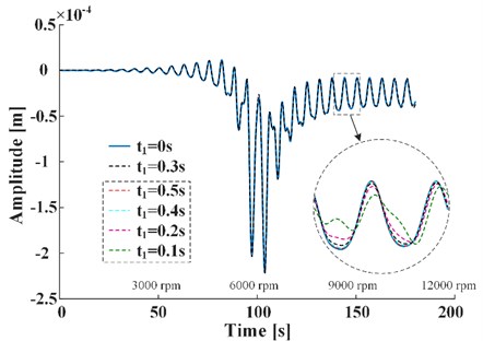
Fig. 5The spectrum transformed by FFT

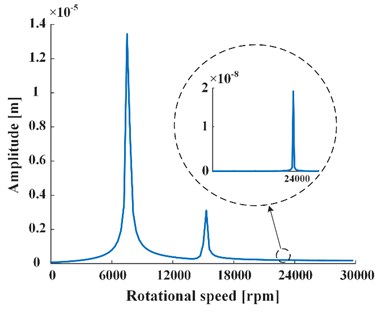
Fig. 6The frequency-response curve of experimental result

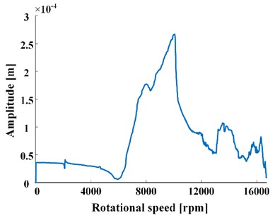
If rotational speed is constant, the amplitudes and phases in Eq. (39) degenerate to constant, which satisfies the time-invariant condition of Fourier transform. As can be seen from Fig. 5 transformed by FFT, the magnitude of the third harmonic generation is three orders of magnitude lower than that of the fundamental frequency. The fundamental frequency is about 8000 rpm, which is a bit consistent with experimental result of speed-up process shown in Fig. 6.

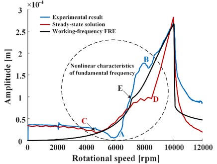
To further verify the nonlinear response characteristics, we put three frequency-response curves, including experimental result, steady-state solution transformed by STFT, working frequency FRE, on the same graph respectively, and intercept the portion of fundamental frequency for comparing, which is shown in Fig. 7. Obviously, all of the curves take on resemblance in the linear vibration features caused by $A_{0} c o s (Ω t + θ_{0})$ . It is worth noting that, the AB segment of experimental result and the CD segment of steady-state solution both present nonlinear vibration characteristics caused by $A_{1} c o s (Ω t + θ_{1})$ . But for the curve of working frequency FRE, there is only one peak point $E$ , which can be considered as an expression of the nonlinear feature, so that it is incomplete and inaccurate to analyze the nonlinear characteristics by just using the working frequency FRE.

Fig. 7Comparison of frequency-response curves

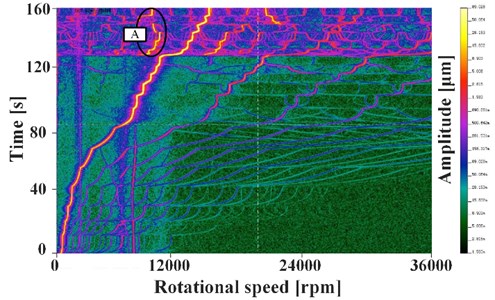
The time-amplitude-frequency spectrum of rotor speed-up process is shown in Fig. 8, and especially in the area A, the whirl starts to appear at the rotational speed of 12487 rpm under the effect of gas film, which due to the fluid-solid coupling mechanism mainly caused by gas bearing used in this experiment. It needs to be noticed that, based on the large deformation and perturbation assumptions, the analytical model in this paper does not consider the subharmonic effect caused by gas film. Additional researches on whirl effect of bearing will be addressed in subsequent work.

Fig. 8Time-amplitude-frequency spectrum of rotor speed-up process

6. Conclusions

In this paper, with respect to reveal the mechanism of dynamic behaviors and nonlinear responses of a rotor system, an analytical model is constructed, and the analytical solutions are derived via multi-scale method. The conclusions are as follows.

1) By defining the nonlinear scale factor $ε$ , and introducing nonlinear stiffness and nonlinear damping, a nonlinear analytical model is presented, which aims to reflect the linear and nonlinear interaction.

2) The analytical solutions of steady-state and transient-state are derived via multi-scale method, and the nonlinear natural frequency and the working frequency FRE are obtained.

3) The mechanism of nonlinear scale factor $ε$ is clarified, which can be used to reflect the degree of influence on nonlinear effects. The rationality and validity of the analytical model are also verified.

4) The transient time scale factor $t_{1}$ is defined to reflect transient-state influence on steady-state, which can be obtained when transient-steady energy ratio decays to 10 %.

5) The steady-state solution well reflects the nonlinear vibration characteristics of the fundamental frequency, which is consistent with the experimental result, rather than that of the working frequency FRE, in which the nonlinear characteristics is represented as one point. Therefore, the rationality of the analytical solutions is verified.

References

Meng G. Retrospect and prospect to the research on rotordynamics. Journal of Vibration Engineering, Vol. 15, Issue 1, 2002, p. 1-9, (in Chinese).

Search CrossRef
Huang W., Wu X., Jiao Y., et al. Review of nonlinear rotor dynamics. Journal of Vibration Engineering, Vol. 13, Issue 4, 2000, p. 497-509, (in Chinese).

Search CrossRef
Yang J., Yang S., Chen C., et al. Research on sliding bearings and rotor system stability. Journal of Aerospace Power, Vol. 23, Issue 8, 2008, p. 1420-1426, (in Chinese).

Search CrossRef
Lund J. W. The stability of an elastic rotor in journal bearings with flexible, damped supports. Journal of Applied Mechanics, Vol. 32, Issue 4, 1965, p. 911-920.

Publisher
Glienicke J. Spring Damping Constants of Turbine Bearings and the Effect on the Vibration Behavior of Single Rotor. Dissertation, TH, Karlsruhe, 1966, (in German).

Search CrossRef
Alford J. S. Protecting turbomachinery from self-excited rotor whirl. Journal of Engineering for Power, Vol. 87, Issue 4, 1965, p. 333-343.

Publisher
Tanaka M., Hori Y. Stability characteristics of floating bush bearings. Journal of Lubrication Technology, Vol. 94, Issue 3, 1972, p. 248-256.

Publisher
Ehrich F. F. High order subharmonic response of high speed rotors in bearing clearance. Journal of Vibration, Acoustics, Stress, and Reliability in Design, Vol. 110, Issue 1, 1988, p. 9-16.

Publisher
Childs D. W. Dynamic analysis of turbulent annular seals based on hirs’ lubrication equation. Journal of Lubrication Technology, Vol. 105, Issue 3, 1983, p. 429-436.

Publisher
Bently D. E., Muszynska A. Role of circumferential flow in the stability of fluid-handling machine rotors. Rotordynamic Instability Problems in High-Performance Turbomachinery (5th), 1988, p. 415-430.

Search CrossRef
Muszynska A., Bently D. E. Anti-swirl arrangements prevent rotor/seal instability. Journal of Vibration, Acoustics, Stress, and Reliability in Design, Vol. 111, Issue 2, 1989, p. 156-162.

Publisher
Ravikovich Yu. A. The Construction and Design of Sliding Bearing Units. Moscow, 1995, (in Russian).

Search CrossRef
Wu M., Yang J. The research on single-disc rotor nonlinear vibration model and mechanism. Mechatronics and Information Technology, PTS 1 and 2, Vols. 2-3, 2012, p. 954-959.

Publisher
Liu B., Peng J. Nonlinear Dynamics. Higher Education Press, Beijing, 2004, (in Chinese).

Search CrossRef
Khalil H. Nonlinear Systems. Electronic Industry Press, Beijing, 2005, (in Chinese).

Search CrossRef
Zhou J., Zhu Y. Nonlinear Vibration. Xi’an Jiaotong University Press, Xi’an, 1998, (in Chinese).

Search CrossRef
Hu H. Nonlinear Vibration. Aviation Industry Press, Beijing, 2000, (in Chinese).

Search CrossRef
Chen Y. Modern Analytical Method in Nonlinear Dynamics. Science Press, Beijing, 1992, (in Chinese).

Search CrossRef
Weng B., Li Y., Xu P. Engineering Nonlinear Vibration. Science Press, Beijing, 2007, (in Chinese).

Search CrossRef
Meng G., Xue Z. Study on nonlinear duffing characteristics of flexible rotor with SFDB. Journal of Aerospace Power, Vol. 4, Issue 2, 1989, p. 173-197, (in Chinese).

Search CrossRef
Han D., Yang J., Chen C., et al. Experimental research on the dynamic characteristics of gas-hybrid bearing-flexible rotor system. Journal of Vibroengineering, Vol. 16, Issue 5, 2014, p. 2363-2374.

Search CrossRef
Han D., Yang J., Zhao C., et al. An experimental study on vibration characteristics for gas bearing-rotor system. Journal of Vibration Engineering, Vol. 25, Issue 6, 2012, p. 680-685, (in Chinese).

Search CrossRef

Cited by

Free Fluid-Structure Interaction Method for Accurate Nonlinear Dynamic Characteristics of the Plain Gas Journal Bearings

Bin Wang | Yongtao Sun | Qian Ding

(2020)

Analytical analysis on damping characteristics of rotor system

Min Wu | Shengbo Yang | Wen Bao | Jinfu Yang

(2017)

About this article

Received

22 July 2016

Accepted

18 November 2016

Published

31 December 2016

SUBJECTS

Mechanical vibrations and applications

DOI

https://doi.org/10.21595/jve.2016.17441

Keywords

flexible rotor system

nonlinear vibration

analytical model

nonlinear scale factor

analytical solution

Acknowledgements

The work is supported by National Science and Technology projects (Grant No. 2012BAA11B02), and the support is gratefully acknowledged.

Author Contributions

Min Wu wrote this paper and take the charge the theoretical work and analysis. Shengbo Yang drew the pictures and a part of the analysis. Dongjiang Han take charge of the experimental work. Daren Yu and Jinfu Yang guide this work, organize the discussion and the analysis.

This is an open access article distributed under the Creative Commons Attribution License, which permits unrestricted use, distribution, and reproduction in any medium, provided the original work is properly cited.

Previous article in issue Previous Next article in issue Next

Research article

2023 08 08

Influence of pivot support stiffness on dynamic characteristics of vertical rotor system

Qirui Liu, Changliang Tang, Tingwei Wu, Yujie Bai

Research article

2023 05 18

Dynamics analysis of the nonlinear rotor system with Geislinger coupling

Jinhong Wang, Zhenping Li, Hongguang Li, Wendi Zhang, Ke Bao

Research article

2019 09 30

An optimized bearing parameter identification approach from vibration response spectra

Rajasekhara Reddy Mutra, Srinivas J

Research article

2018 12 31

Stability and bifurcation of a flexible rod-fastening rotor bearing system with a transverse open crack

Nanshan Wang, Heng Liu, Yi Liu, Zhidong Xu

M. Wu, S. Yang, D. Han, D. Yu, and J. Yang, “Analytical model for nonlinear vibration of flexible rotor system,” Journal of Vibroengineering, Vol. 18, No. 8, pp. 4980–4994, Dec. 2016, https://doi.org/10.21595/jve.2016.17441

Copy Extrica

Copied to clipboard!

TY  - JOUR
DO  - 10.21595/jve.2016.17441
UR  - https://doi.org/10.21595/jve.2016.17441
TI  - Analytical model for nonlinear vibration of flexible rotor system
T2  - Journal of Vibroengineering
AU  - Wu, Min
AU  - Yang, Shengbo
AU  - Han, Dongjiang
AU  - Yu, Daren
AU  - Yang, Jinfu
PY  - 2016
DA  - 2016/12/31
PB  - JVE International Ltd.
SP  - 4980-4994
IS  - 8
VL  - 18
SN  - 1392-8716
ER  - 

Copy Ris

Copied to clipboard!

@article{Wu_2016,
	doi = {10.21595/jve.2016.17441},
	url = {https://doi.org/10.21595/jve.2016.17441},
	year = 2016,
	month = {dec},
	publisher = {{JVE} International Ltd.},
	volume = {18},
	number = {8},
	pages = {4980--4994},
	author = {Min Wu and Shengbo Yang and Dongjiang Han and Daren Yu and Jinfu Yang},
	title = {Analytical model for nonlinear vibration of flexible rotor system},
	journal = {Journal of Vibroengineering}
}

Copy Bibtex

Copied to clipboard!

[1]M. Wu, S. Yang, D. Han, D. Yu, and J. Yang, “Analytical model for nonlinear vibration of flexible rotor system,” Journal of Vibroengineering, vol. 18, no. 8, pp. 4980–4994, Dec. 2016, doi: 10.21595/jve.2016.17441.

Copy IEEE

Copied to clipboard!

Wu, Min, Shengbo Yang, Dongjiang Han, Daren Yu, and Jinfu Yang. “Analytical Model for Nonlinear Vibration of Flexible Rotor System.” Journal of Vibroengineering 18, no. 8 (December 31, 2016): 4980–94. https://doi.org/10.21595/jve.2016.17441.

Copy Chicago

Copied to clipboard!

Analytical model for nonlinear vibration of flexible rotor system

Abstract

1. Introduction

2. Model formulation

2.1. Nonlinear stiffness

2.2. Nonlinear damping

2.3. Analytical model

3. Analytical solutions and analysis

3.1. Free vibration mode

3.2. Forced vibration mode

3.3. Frequency response equation (FRE)

4. Experimental Facility and procedure

5. Results and discussion

6. Conclusions

References

Cited by

About this article

Related Articles