Abstract
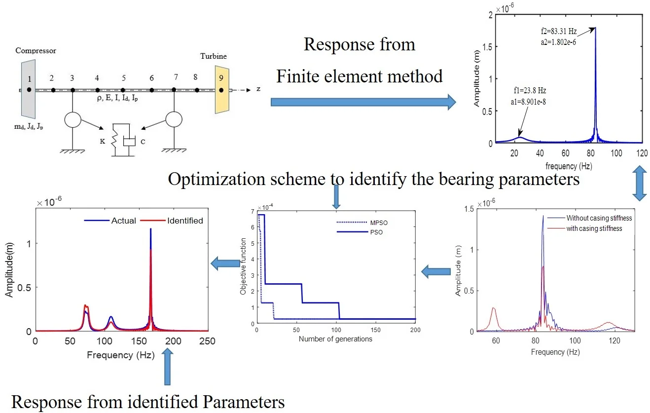
In the present work, an effective identification methodology bearing dynamic parameters using measured vibration responses at the bearing is proposed. The flexible rotor is analyzed by using finite element beam model with nonlinear hydrodynamic bearing forces due to floating ring bearing supports. The frequency domain responses at different operating speeds are initially obtained in both the lateral directions. The error function is formulated as an average difference in amplitudes of two lateral displacements at a bearing node with known reference signals over a frequency range. The design variables are the speed dependent direct and cross-coupled stiffness and damping parameters of the bearing. With the side constraints on the variables, the error is minimized by using a modified particle swarm optimization scheme. The accuracy of the approach is tested with noisy input signals.
Highlights
- Identification of the unknown bearing stiffness and damping coefficients from the known responses in a less computational time
- Measurements of lateral displacements at the bearings are simultaneously taken to achieve more accuracy in identification of parameters
- Objective function considered is the sum of the mean square errors of displacements in both directions
- Cross-coupled stiffness and damping coefficients are also calculated at the two bearings
- The effect of stiffness of the bearing casing is accounted for obtaining the dynamic responses
1. Introduction
Identification of rotor bearing parameters is an essential task in simplifying stability analysis procedure. Especially, the bearing parameters drastically affect vibration modes and responses of a rotating system. In practice, the high-speed rotors are often supported on various types of bearings and have unbalance and coupling forces leading to complex overall dynamics. Nowadays, the fluid film bearings are widely used in such rotors in reducing critical vibration amplitudes considerably due to their high damping and stiffness forces. These time-varying supporting forces often result in highly nonlinear response signals. Moreover, such force systems employ considerable computational memory which leads to relatively slower output performances. Equivalent linear bearing parameters if identified on the other way would result in better outcomes with respect to computational requirements. Further, these parameters are speed dependent [1] and require careful identification approaches. The identification studies of bearing parameters have been presented widely for plain and aerostatic journal bearings [2-4] estimated linear and nonlinear bearing stiffness of journal bearing using perturbation technique with two-dimensional Newton-Raphson iteration method. The methodology of prediction of sixteen dynamic coefficients for journal bearings in a rotor system from experimental unbalance responses was presented in Ref. [5, 6]. A method with multi-frequency excitation for measurement of equivalent stiffness and damping of the active magnetic bearing rotor was presented [7]. From the unbalance response [8, 9] and frequency characteristics [10], similar kinds of magnetic bearing parameter identification approaches were found. For ball bearing systems, the parameters were identified with simulated and experimental data [11]. Linear and nonlinear bearing coefficients of oil-free bearings including gas-foil [12-16] and gas-film bearings [17, 18] were obtained. Response based identification methodologies for tilting pad journal bearings were also noticed [19-21].
Hydrodynamic bearing forces are highly nonlinear and parametric in nature. For hydrodynamic journal bearings, field identification method for stiffness and damping characteristics was illustrated [22] using measured responses at both shaft and housing locations. An experimental approach was proposed [23] to estimate the stiffness and damping parameters via the least-square minimization under different operating conditions. A procedure to evaluate the rotor dynamic force coefficients of series bearing-supports was presented for impact and unbalance from the field measurements [24]. For identification of bearing parameters and unbalance from the measured responses, an optimization based strategy was proposed [25]. Qu et al. [26] explained the influence of the support stiffness on the engine vibration characteristics. Kriging surrogate model together with differential evolution optimization scheme was implemented [27, 28] to predict the bearing parameters. A modal parameter genetic time domain identification approach has been proposed [29] to study the characteristics of bearings using a multi-frequency signal decomposition technic. Prediction of bearing parameter information chart is; therefore, a very important task and a generalized methodology is, therefore, necessary to obtain the parameters conveniently. Although many studies are available in the literature, the estimation approaches based on correlating the real-time data with model-based outputs are found in limited papers. In the present work, the speed-dependent stiffness and damping parameters of the floating-ring bearing system are obtained from frequency response measurements followed by minimizing the average error in amplitudes between the actual and model-based response signals. Initially, the reference signal is obtained by analyzing the rotor-bearing system using three-dimensional beam element model of a rotor supported over floating ring bearings. The speed-dependent bearing coefficients are considered as variables and MPSO scheme is implemented to minimize the mean square error between the reference and linear idealized signals. Robustness of methodology is tested by introducing the noise into the measured reference signal. The main focus of this work is obtaining the unknown bearing stiffness and damping coefficients from the known responses in a less computational time. Measurements of lateral displacements at the bearings are simultaneously taken to achieve more accuracy in identification of parameters. Objective function considered is the sum of the mean square errors of displacements in both directions. Cross-coupled stiffness and damping coefficients are also calculated at the two bearings. In addition, the effect of stiffness of the bearing casing is accounted for obtaining the dynamic responses.
Remaining part of the paper is organized as follows: Section 2 describes the rotor-bearing system model and the expression of nonlinear bearing forces as well as the dynamic formulation of equivalent lumped parameter model of the rotor-bearing system. Section 3 presents the formulation of the objective function and optimization technique employed in the present work. Finally, the model validation along with optimization outcomes of a test case is illustrated in the results and discussion part.
2. Dynamic model of rotor bearing system
The more effective advantage of supporting action can be obtained at high speeds from dual-film hydrodynamic bearing systems such as full and semi floating-ring bearings. The response studies in high-speed rotor dynamic systems with floating ring journal bearings were thoroughly analyzed by simplified mathematical models [30-33]. The dynamic model of the flexible rotor dynamic system is formulated using quasi-finite element analysis with lumped floating ring masses considered at the bearing locations. The shaft is treated as flexible member and disks are treated as rigid. Each node has four degrees of freedom (DOF) including two translations (, ) and two bending slopes (, ). By consideration of the bending and shearing effects the kinetic and potential energy of the shaft element can be expressed as:
The kinetic energy of each disk can be expressed as:
The virtual work done by unbalance forces at the disks can be expressed as:
From Hamilton principle:
with denotes the variational symbol, the equations of motion of the rotor alone is written as:
where, represents the displacement vector of size , represents both the unbalance force and gravity force vector at the disks. is the inner oil film force and , , and denote respectively the assembled system mass, system damping, gyroscopic matrix of shaft and stiffness matrices assembly of size . The motion of the floating ring is identified with the help of inner and outer oil film hydrodynamic fluid forces, feed pressure of the lubricant and floating ring dead weight. The final motion of equation for the floating ring is written as:
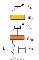
where denotes the 4×1 displacement vector of the floating rings at both bearings, is the mass matrix of the rings with size 4×4. The outer and inner oil film forces of floating ring bearing can be represented as and . By accounting the housing flexibility in the form of a single degree of freedom model with fixed mass, stiffness and damping coefficients, the combined simplified system is shown in Fig. 1.
Fig. 1Combined floating ring bearing forces with housing
The equation of motion of bearing housing of floating-ring is represented as:
where:
are the corresponding 4×4 mass, damping and stiffness matrices of the bearing housings at both left and right bearings, denotes the 4×1 displacement vector of the bearing housings. By combining the system of equations for rotor and bearing, the assembled equations are represented as:
where:
are effective square matrices, while is vector of displacements and is resultant force vector of unbalance, bearing and gravity forces.
2.1. Floating-ring bearing with elastic housing
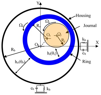
A floating ring bearing (FRB) has an annular ring placed in-between the journal and sleeve and there is a thin oil film in-between them. The bearing mid-plane consists of the circumferential feed grooves and the lubricant is fed from the journal to the sleeve via a bunch of feed holes located in the ring. The coordinate system considered is shown in Fig. 2.
Fig. 2Geometry of the floating-ring bearing with housing elasticity
With the help of the film pressure distribution, the hydrodynamic fluid forces can be derived from 2-D Reynold’s equation. Reynolds equations for both inner and outer lubricant films can be expressed as follows:
where is the pressure of the oil film, and represents the viscosity of the lubricating oil, the subscripts and denote the parameters of inner oil film and outer oil film, respectively. While the subscripts and indicate the parameters between the journal and floating ring. and correspond to the journal and floating ring outer radius, respectively. is the angular coordinate for the inner and outer oil films. The axial coordinates of the inner and outer films are denoted by and respectively. The simplified expressions for oil film thicknesses and the film pressure distributions are expressed by considering Octvick’s theory of short bearings as:
where (, ) is the displacement vector of the journal center in the fixed reference frame. Also, and represent the static clearances of inner and outer film regions. The absolute displacement and velocity components of the floating ring center are (, ) and (, ) while the absolute velocities of centers are denoted as . The lower case letters , (, ) denote the displacement and velocity components of relative to . The final expressions for inner and outer oil film force components are written as [34]:
where the detailed expression for ,,, are given in the Appendix.
3. Methodology and optimization technique
The bearing force components are expressed in terms of displacements and velocities in bearing coordinates as:
where the terms and represent the unknown damping and stiffness bearing force coefficients. The direct and cross-coupled terms are denoted by suffices , and respectively. The suffix denotes the bearing support location. By substituting these bearing forces into the Eq. (9) and converting to the frequency domain, the system of equations can be rewritten as:
where, is impedance function, (, ) and (, ) are the discrete Fourier transforms of external forces and displacements respectively. With the knowledge of the component displacements in bending directions at any location on the rotor, it is possible to compute the twelve force coefficients corresponding to each of the two bearings. In order to obtain the correct set of parameters, an error function defined in terms of and amplitudes at the bearing nodes is considered at every operating speed. Mathematical formulation of the optimization problem in the current context is stated as:
where and are the reference amplitudes obtained from the nonlinear force model, while and are the corresponding displacement amplitude of frequency response via linear bearing forces. Here, denotes the total number of sample points considered in frequency-domain. This error is an implicit function of bearing coefficients which are defined with upper and lower bounds.
3.1. Particle swarm optimization (MPSO) with mutation
Conventional particle swarm optimization scheme is one of the robust metaheuristic optimization methods works on the behavior of flocking birds/fish during the food search [35]. Initially, with the random set of solutions, the system starts and searches for optimum value by updating the generations. The particle is described as each candidate solution and set of particles is known as a swarm. In a cooperative manner, they move in n-dimensional search space. The variable velocity performs the swarm movement of each particle. This velocity is influenced by social and local factors. Each particle moves through the search space based on the best positions found so far by itself ()and the best position found by the swarm (). In search space (with initial sets) for each particle, the objective function value is calculated. If and are position and velocity of each particle at thiteration, movements of each particle are influenced by three factors (i) own direction search of Particle (ii) Particle beast position itself (iii) whole swarms best position. The position and velocity of every particle after iteration number is updated using the following equation:
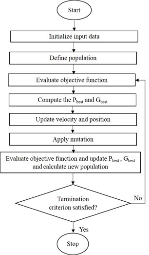
where is called inertia factor of the particle, which often reduced in every cycle. Acceleration coefficients and describe the private (cognitive) and global (social) behavior of the system. Also, and are random numbers between 0 and 1. is the best position of particle till the current iteration while is the best position of the group until current iteration. The algorithm converges to the best swarm by selecting the correct values of , and . Further, the velocity of the particle is bounded between the minimum and maximum values. Premature convergence can take place under different situations such as (i) the population has converged to local optima, (ii) the population has lost its diversity resulting in the search algorithm to proceed slowly. In this regard, to attain faster convergence without loss of accuracy, several modifications were suggested. To improve the population diversity and PSO’s performance, mutation is a powerful tool [36]. Here, a correction to the updated vector in every cycle is introduced. This approach evaluates a mutation vector created from randomly selected three swarms (vectors, , and ) in that generation. Fig. 3 shows the flowchart of the MPSO approach. The termination criterion employed in the present work is to achieve the maximum number of generations or to attain the error tolerance in successive objective function values whichever reaches earlier.
Mathematically, mutation vector () is expressed as [37]:
where [0.9, 1] is the mutation constant.
The resultant population is modified using this mutation vector according to the following rule:
Here, is the number of points in the population (swarm size). The is crossover probability selected in the range of 0.1 to 0.9.
Fig. 3Flowchart of MPSO
4. Results and discussion
In order to examine the potentiality of the objective function, the simulated frequency response is initially generated from the rotor system with a linear bearing model having certain known input bearing force coefficients. This reference signal with input bearing force coefficients is provided to the optimization program and the bearing parameters are retrieved back through the error minimization procedure. The rotor is analyzed by finite element model using Timoshenko beam elements having two bending deflections and slopes at each node.
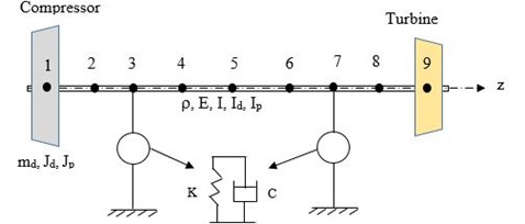
There are eight elements and nine nodes and total degrees of freedom are equal to 36. The discs are mounted at nodes 1 and 9, while the bearing nodes are at 3 and 7 as shown in Fig. 4.
Fig. 4Finite element model of the rotor- bearing system
Dimensional data of the rotor system is represented in Table 1.
Table 1Dimensional date of rotor system [32]
Properties | Value |
Shaft material density (kg/m3) | 7800 |
Left disk mass (kg) | 1.4 |
Right disk mass, (kg) | 1 |
Left disk diameter moment of inertia, (kgm-2) | 6.3×10⁻⁴ |
Right disk diameter moment of inertia, (kgm-2) | 4.5×10⁻⁴ |
Left disk polar moment of inertia, (kgm-2) | 1.26×10⁻⁵ |
Right disk polar moment of inertia, (kgm-2) | 9×10⁻⁴ |
Rotor diameter, (m) | 0.02 |
Rotor length, (m) | 0.4 |
Young’s modulus, (GPa) | 200 |
Radius of bearing (m) | 0.01 |
Length of bearing (m) | 0.01 |
Radial clearance of bearing (microns) | 200 |
Viscosity of Oil film (Pa-s) | 288×10-4 |
Eccentricity (m) | 1×10⁻⁶ |
The dynamic equations are solved by using fourth order Runge-Kutta time integration method with zero initial conditions. Fig. 5 shows the frequency response obtained at the left bearing node at a rotor speed of 5000 rpm. As the peak modes are occurring over the range 0-100 Hz, within this span the amplitudes are accounted in the objective function.
Fig. 5Frequency domain response at left bearing (kxx= 0.25 Mn/m, kxy= 0.12 Mn/m, kyy= 0.275 Mn/m, cxx= 300 Ns/m, cxy= 20 Ns/m, cyy= 399 Ns/m)
a)-direction
b)-direction
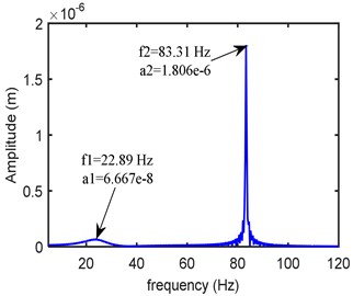
The PSO parameters are taken as: 2.1 and , where is maximum weight, is minimum weight, is iteration number and is maximum iterations. In present study, 0.9 and 0.4. The variable bounds are taken as: [10 kN/m, 5 MN/m], [10 N-s/m, 5000 N-s/m]. Fig. 6 shows the final error achieved for different swarm sizes at a rotor speed 5000 rpm. The minimum error occurs at a swarm size of 30.
Fig. 7 shows the fitness function convergence using proposed MPSO with a swarm size of 30 along with standard PSO scheme. It is seen that MPSO converges at a faster rate.
Table 2 shows the obtained bearing parameters as optimized design variables. The identified direct and cross-coupled parameters are found close to the reference values. Furthermore, the noise is added to the response signal for predicting the accuracy of identification. In this regard, random signal is added as a fraction of original signal. The percentage deviation is relatively small with the added input noise the frequency response.
Fig. 6Effect of swarm size in MPSO on converged error
Fig. 7Objective function convergence in PSO and MPSO
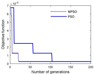
Table 2Assumed and estimated bearing parameters for linear rotor model
Parameter | Reference values | Without noise | With 5 % noise | With 10 % noise |
×10-5 (N/m) | 2.50 | 2.532 | 2.554 | 2.591 |
×10-5 (N/m) | 1.20 | 1.211 | 1.218 | 1.221 |
×10-5 (N/m) | 2.75 | 2.763 | 2.799 | 2.825 |
×10-5 (N/m) | 2.75 | 2.778 | 2.785 | 2.798 |
×10-5 (N/m) | 1.46 | 1.465 | 1.476 | 1.483 |
×10-5 (N/m) | 2.82 | 2.832 | 2.892 | 2.934 |
(Ns/m) | 300 | 303.24 | 303.94 | 304.64 |
(Ns/m) | 20 | 20.12 | 20.69 | 20.94 |
(Ns/m) | 399 | 400.91 | 401.15 | 402.27 |
(Ns/m) | 315 | 316.98 | 317.84 | 319.58 |
(Ns/m) | 59 | 59.25 | 59.64 | 59.92 |
(Ns/m) | 300 | 302.54 | 302.81 | 303.47 |
4.1. Rotor supported on floating-ring bearings
With floating ring nonlinear bearing forces, the rotor response is obtained from the same finite element model of the rotor. This time, the speed-varying equivalent bearing force parameters are obtained. Table 3 shows the bearing parameters employed in the simulation.
Table 3Floating-ring bearing parameters considered [32]
Parameter | Value |
Bearing outer clearance (m) | 8×10⁻⁵ |
Bearing inner clearance (m) | 2×10⁻⁵ |
Mass of the ring (kg) | 0.02 |
Inner film viscosity (Pa-s) | 0.006 |
Outer film viscosity (Pa-s) | 0.012 |
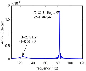
The time responses and frequency spectra in two directions are obtained at different operating speeds. The stiffness, damping, and mass of the bearing casing are respectively considered as 100 kN/m, 100 Ns/m and 0.1 kg. Fig. 8 shows the frequency spectra at a speed of 5000 rpm with and without accounting the casing stiffness. It is seen that there are two critical frequencies (at 83 Hz and 120 Hz) in the first case without casing flexibility. Furthermore, the subharmonic resonances resulting from hydrodynamic bearing forces are relatively small at this speed of operation [38]. With casing flexibility taken into account, it is observed that an additional mode is each direction results. The amplitude of the main dominating peak became small in both the directions as an absorber effect.
In order to identify the bearing coefficients, the response data is given as input to the optimization program. The same error function is further minimized by other well-known meta-heuristic optimization methods namely genetic algorithms (GA) [39] and simulated annealing (SA) [40]. In GA, population sizes of 30 along with mutation and crossover functions selected as constraint dependent and scattered type respectively. In SA also the function tolerance is considered as 10-6. The annealing function used is fast annealing type and the reannealing interval considered as 100. The error function value obtained, and computation time taken in all three approaches are depicted in Table 4.
Fig. 8Frequency spectra at left bearing
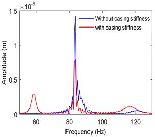
a)-direction
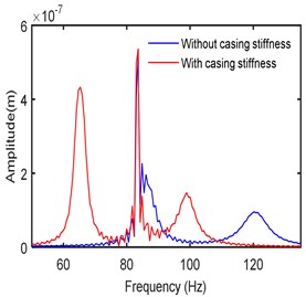
b)-direction
Table 4Performance comparison of various optimization schemes
Method | Error | Time (s) |
MPSO | 5.49e-17 | 140 |
GA | 1.083e-14 | 155 |
SA | 1.082e-11 | 185 |
It is seen that the MPSO is relatively good in terms of both accuracy and computational time. Table 5 shows the identified bearing stiffness coefficients at different operating speeds obtained from MPSO.
The corresponding identified damping parameters are given in Table 6.
Table 7 shows changes in the identified parameters at a rotor speed of 10,000 rpm with added noise in the frequency response. It is observed that the average error is well below 4 %.
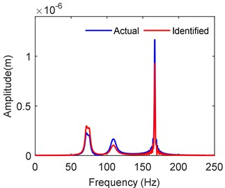
Using the identified parameter data, the response at the left bearing node is further obtained from the finite element model and is shown in Fig. 9. The corresponding response with floating ring bearing forces at 10,000 rpm is also illustrated for comparison. The response spectrum is well matching with marked resonant peaks.
Table 5Identified stiffness coefficients of the bearings at different speeds
Sl. No | Speed (rpm) | Bearing-1 | Bearing-2 | ||||
(MN/m) | (MN/m) | (MN/m) | (MN/m) | (MN/m) | (MN/m) | ||
1 | 1000 | 3.1501 | 3.43912 | 1.2102 | 2.916827 | 3.145741 | 1.4651 |
2 | 2000 | 3.0110 | 3.45786 | 1.2113 | 2.81801 | 3.31343 | 1.4865 |
3 | 3000 | 3.0011 | 3.81297 | 1.2236 | 2.803257 | 3.621957 | 1.5135 |
4 | 4000 | 3.0001 | 4.16761 | 1.2258 | 2.758222 | 3.681405 | 1.5364 |
5 | 5000 | 2.9140 | 4.37417 | 1.3451 | 2.637015 | 3.83408 | 1.5412 |
6 | 6000 | 2.8466 | 4.62592 | 1.8684 | 2.45915 | 4.086198 | 1.5945 |
7 | 7000 | 2.8141 | 4.88159 | 2.2687 | 2.38048 | 4.15605 | 1.6124 |
8 | 8000 | 2.7957 | 5.27948 | 2.5587 | 2.193331 | 4.234727 | 1.6354 |
9 | 9000 | 2.8511 | 5.67308 | 2.6869 | 2.043291 | 4.327847 | 1.6589 |
10 | 10000 | 2.9534 | 5.95391 | 2.7246 | 2.006007 | 4.543091 | 1.6758 |
Table 6Identified damping coefficients of the bearings at different speeds
Sl.no | Speed (rpm) | Bearing-1 | Bearing-2 | ||||
(MNs/m) | (MNs/m) | (MNs/m) | (MNs/m) | (MNs/m) | (MNs/m) | ||
1 | 1000 | 0.00434 | 0.0049 | 0.00028 | 0.004291 | 0.004923 | 0.00035 |
2 | 2000 | 0.004238 | 0.00479 | 0.00029 | 0.003912 | 0.004835 | 0.00036 |
3 | 3000 | 0.004138 | 0.00492 | 0.00031 | 0.003839 | 0.004723 | 0.00039 |
4 | 4000 | 0.003924 | 0.0050 | 0.00035 | 0.003792 | 0.004957 | 0.00041 |
5 | 5000 | 0.003748 | 0.00511 | 0.00039 | 0.004001 | 0.005085 | 0.00042 |
6 | 6000 | 0.00386 | 0.00549 | 0.00041 | 0.004182 | 0.00533 | 0.00043 |
7 | 7000 | 0.00398 | 0.00568 | 0.00043 | 0.004314 | 0.005711 | 0.00046 |
8 | 8000 | 0.004002 | 0.00583 | 0.00043 | 0.004408 | 0.005877 | 0.00049 |
9 | 9000 | 0.004149 | 0.00606 | 0.00043 | 0.004693 | 0.005916 | 0.00050 |
10 | 10000 | 0.004316 | 0.00627 | 0.00043 | 0.004942 | 0.006178 | 0.00512 |
Table 7Identified bearing parameters with added noise at 10,000 rpm
Parameter | Without noise | With 5 % noise | With 10 % noise |
(MN/m) | 2.9534 | 2.974 | 2.991 |
(MN/m) | 2.7246 | 2.754 | 2.785 |
(MN/m) | 5.95391 | 5.995 | 6.024 |
(MN/m) | 2.00600 | 2.012 | 2.098 |
(MN/m) | 1.6758 | 1.694 | 1.701 |
(MN/m) | 4.543091 | 4.578 | 4.597 |
(MNs/m) | 0.004316 | 0.00451 | 0.0047 |
(MNs/m) | 0.00043 | 0.00047 | 0.0005 |
(MNs/m) | 0.00627 | 0.00635 | 0.0064 |
(MNs/m) | 0.004942 | 0.00501 | 0.0052 |
(MNs/m) | 0.00512 | 0.00534 | 0.0054 |
(MNs/m) | 0.006178 | 0.00628 | 0.0064 |
Fig. 9Comparison of frequency response at left bearing node (10,000 rpm)
5. Conclusions
In this work, bearing force parameter identification procedure was illustrated with available frequency spectra in a rotor dynamic system. Flexible rotor system was analyzed by using a finite element model and the frequency domain responses at different rotor speeds were considered. An error-based formulation in terms of response amplitudes at bearing nodes was employed and the speed dependent stiffness and damping parameters of the bearings were identified via modified particle swarm optimization with the mutation. The methodology was found to be reliable and predicts the coefficients with limited computation effort. Robustness of methodology was tested by introducing the noise into the measured reference signals. The average error was not exceeding four percent. The average time for function evaluation can be further minimized by employing an approximate solution technique for solving nonlinear dynamic equations for achieving directly the frequency spectrum without the need of time domain analysis. Alternatively, surrogate models via neural networks may also be employed to avoid the complex time-domain calculations.
References
-
Tiwari R., Lees A. W., Friswell M. I. Identification of dynamic bearing parameters: a review. The Shock and Vibration Digest, Vol. 36, 2004, p. 99-124.
-
Meruane V., Pascual R. Identification of nonlinear dynamic coefficients in plain journal bearings. Tribology International, Vol. 41, 2008, p. 743-754.
-
Kozánek J., Šimek J., Steinbauer P., Bílkovský A. Identification of stiffness and damping coefficients of aerostatic journal bearing. Engineering Mechanics, Vol. 16, 2009, p. 209-20.
-
Choy F. K., Braun M. J., Hu Y. Nonlinear effects in a plain journal bearing: part 1 – analytical study. Journal of Tribology, Vol. 113, 1991, p. 555-561.
-
Tieu A. K., Qiu Z. L. Identification of sixteen dynamic coefficients of two journal bearings from experimental unbalance responses. Wear, Vol. 177, 1994, p. 63-69.
-
Qiu Z. L., Tieu A. K. Identification of sixteen force coefficients of two journal bearings from impulse responses. Wear, Vol. 212, 1997, p. 206-212.
-
Jiang K., Zhu C., Chen L., Qiao X. Multi-DOF rotor model-based measurement of stiffness and damping for active magnetic bearing using multi-frequency excitation. Mechanical Systems and Signal Processing, Vol. 60, Issue 61, 2015, p. 358-374.
-
Zhou J., Di L., Cheng C., Xu Y., Lin Z. A rotor unbalance response based approach to the identification of the closed-loop stiffness and damping coefficients of active magnetic bearings. Mechanical Systems and Signal Processing, Vols. 66-67, 2016, p. 665-78.
-
Xu Y., Zhou J., Di L., Zhao C. Active magnetic bearings dynamic parameters identification from experimental rotor unbalance response. Mechanical Systems and Signal Processing, Vol. 83, 2017, p. 228-240.
-
Jin C., Xu Y., Zhou J., Cheng C. Active magnetic bearings stiffness and damping identification from frequency characteristics of control system. Shock and Vibration, Vol. 2016, 2016, p. 1067506.
-
Jacobs W., Boonen R., Sas P., Moens D. The influence of the lubricant film on the stiffness and damping characteristics of a deep groove ball bearing, Mechanical Systems and Signal Processing, Vol. 42, 2014, p. 335-350.
-
Peng J. P., Carpino M. Calculation of stiffness and damping coefficients for elastically supported gas foil bearings. Journal of Tribology, Vol. 115, 1993, p. 20-27.
-
San Andrés L., Chirathadam T. A., Kim T. H. Measurement of structural stiffness and damping coefficients in a metal mesh foil bearing. Journal of Engineering for Gas Turbines and Power, Vol. 132, 2009, p. 032503.
-
Arora V., Hoogt Van Der P. J. M., Aarts R. G. K. M., Boer De A. Identification of stiffness and damping characteristics of axial air-foil bearings. International Journal of Mechanics and Materials in Design, Vol. 7, 2011, p. 231-243.
-
Zhang B., Qi S., Feng S., Geng H., Sun Y., Yu L. An experimental investigation of a microturbine simulated rotor supported on multileaf gas foil bearings with backing bump foils. Proceedings of the Institution of Mechanical Engineers, Part J: Journal of Engineering Tribology, Vol. 232, Issue 9, 2017, p. 1169-1180.
-
Wilkes J. C., Wade J., Rimpel A., Moore J., Swanson E., Grieco J., et al. Impact of bearing clearance on measured stiffness and damping coefficients and thermal performance of a high-stiffness generation 3 foil journal bearing. ASME Turbo Expo 2016: Turbomachinery Technical Conference, 2016.
-
Czołczyński K. How to obtain stiffness and damping coefficients of gas bearings. Wear, Vol. 201, 1996, p. 265-275.
-
Dellacorte C. Stiffness and damping coefficient estimation of compliant surface gas bearings for oil-free turbomachinery. Tribology Transactions, Vol. 54, 2011, p. 674-684.
-
Asgharifard Sharabiani P., Ahmadian H. Nonlinear model identification of oil-lubricated tilting pad bearings. Tribology International, Vol. 92, 2015, p. 533-543.
-
Theisen L. R. S., Niemann H. H., Santos I. F., Galeazzi R., Blanke M. Modelling and identification for control of gas bearings. Mechanical Systems and Signal Processing, Vol. 70, Issue 71, 2016, p. 1150-1170.
-
Wang W., Liu B., Zhang Y., Shao X., Allaire P. E. Theoretical and experimental study on the static and dynamic characteristics of tilting-pad thrust bearing. Tribology International, Vol. 123, 2018, p. 26-36.
-
Tawfick S. H., El Shafei A., Mokhtar M. O. A. Field identification of stiffness and damping characteristics of fluid film bearings. ASME Turbo Expo 2008: Power for Land, Sea and Air, Vol. 5, 2008, p. 1191-1201.
-
Zhou H., Zhao S., Xu H., Zhu J. An experimental study on oil-film dynamic coefficients. Tribology International, Vol. 37, 2004, p. 245-253.
-
De Santiago O. C., San Andrés L. Field methods for identification of bearing support parameters –part I: identification from transient rotor dynamic response due to impacts. Journal of Engineering for Gas Turbines and Power, Vol. 129, 2007, p. 509-517.
-
Kim Y. H., Yang B. S., Tan A. C. C. Bearing parameter identification of rotor–bearing system using clustering-based hybrid evolutionary algorithm. Structural and Multidisciplinary Optimization, Vol. 33, 2007, p. 493-506.
-
Qu M., Chen G., Tai J. Influence of support stiffness on aero-engine coupling vibration quantitative analysis. Journal of Vibroengineering, Vol. 19, Issue 8, 2017, p. 5746-5757.
-
Han F., Guo X., Gao H. Bearing parameter identification of rotor-bearing system based on Kriging surrogate model and evolutionary algorithm. Journal of Sound and Vibration, Vol. 332, 2013, p. 2659-2671.
-
Han F., Guo X., Mo C., Gao H., Hou P. Parameter identification of nonlinear rotor-bearing system based on improved kriging surrogate model. Journal of Vibration and Control, Vol. 23, 2017, p. 794-807.
-
Song Z., Liu Y. Dynamic parameter identification of hydrodynamic bearing-rotor system. Shock and Vibration, Vol. 2015, 2015, p. 959568.
-
Li C. H. Dynamics of rotor bearing systems supported by floating ring bearings. Journal of Lubrication Technology, Vol. 104, 1982, p. 469-476.
-
Zhang H., Shi Z. Q., Zhen D., Gu F. S., Ball A. D. Stability analysis of a turbocharger rotor system supported on floating ring bearings. Journal of Physics: Conference Series, Vol. 364, 2012, p. 012032.
-
Hao Zhang, Zhanqun Shi, Shunxin Zhang, Fengshou Gu, Andrew Ball Stability analysis for a turbocharger rotor system under nonlinear hydrodynamic forces. Scientific Research and Essays, Vol. 8, 2013, p. 1495-1511.
-
Wang L., Bin G., Li X., Zhang X. Effects of floating ring bearing manufacturing tolerance clearances on the dynamic characteristics for turbocharger. Chinese Journal of Mechanical Engineering, Vol. 28, 2015, p. 530-540.
-
Adiletta G., Guido A. R., Rossi C. Chaotic motions of a rigid rotor in short journal bearings. Nonlinear Dynamics, Vol. 10, 1996, p. 251-269.
-
Eberhart R., Kennedy J. A new optimizer using particle swarm theory. Proceedings of the 6th International Symposium on Micro Machine and Human Science, 1995.
-
Hu X., Eberhart R. C., Shi Y. Swarm intelligence for permutation optimization: a case study of n-queens problem. Proceedings of the IEEE Swarm Intelligence Symposium, 2003.
-
Kaboli M., Ghanavati B., Akhlaghi M. New CMOS pseudo approximation exponential function generator by modified particle swarm optimization algorithm. Integration, the VLSI Journal, Vol. 56, 2017, p. 70-76.
-
Rao J. S. Rotor Dynamics. New Age International, 1996.
-
Deb K. Optimization for Engineering Design: Algorithms and Examples. Prentice-Hall of India, 2004.
-
Kirkpatrick S., Gelatt C. D., Vecchi M. P. Optimization by simulated annealing. Science, Vol. 220, 1983, p. 671-680.
Cited by
About this article

The authors are grateful to the National Institute of Technology, Rourkela, Odisha, India for extending their facilities to carry out the research work.
