Abstract
Based on the typical start and stop conditions of aeroengine high pressure rotor, the problem of flow-thermo-elastic coupling is solved in this research. Applying basic theory and control equation, it is analyzed the fields of transient temperature, thermal stress and thermal deformation in the start and stop process. Then the temperature at last stopping moment is selected as the boundary condition. With the flow-thermo-elastic coupling method, the distributions of air flow, heat transfer and temperature are discussed in high pressure rotor cavity. The results show the rotor has a higher temperature, and the density of temperature contour is much larger at the beginning of stop period. The temperature of each node gradually decreases as stop time increases. When the stop time is within 40-90 minutes, temperature difference between the upper and lower surfaces is larger than 20 °C. The distribution of transient temperature is different when restart process is taken at different stop moments. If the stop time is short, temperature distribution of the rotor is decreased firstly, then increased, and finally decreased. The time corresponding to the lowest temperature is also different in each node. It is the longest in the 3rd disk, and the shortest in the 8th disk.
Highlights
- With the flow-thermo-elastic coupling method, distributions of air flow, heat transfer and temperature are discussed.
- The density of temperature contour is much larger at the beginning of stop period.
- The distribution of transient temperature is different when restart process is taken at different stop moments.
- If stop time is short, temperature distribution of the rotor is decreased firstly, then increased, and finally decreased.
1. Introduction
Vibration response caused by thermal bending is a more common failure of aeroengine rotor system [1, 2]. Thermal bending usually occurs at the cool state when engine rotor is stopped. Due to the high temperature of engine rotor, the cavity airflow is dissipated to the surrounding environment in a natural convection manner, until it reaches the equilibrium with ambient temperature. For engine rotor, the thickness of boundary layer formed by natural convection tends to be thin below and thick above. Hence, the coefficient of heat transfer is the largest at the lower side of rotor cross section. It gradually decreases along the upward direction of rotor surface.
With the consuming of time, temperature below the rotor is lower due to the faster heat dissipation, and the upper part is opposite. In this way, a temperature difference is formed between the upper surface and the lower surface. So, it is resulted in a thermal bending deformation of the rotor. When the rotor is hot started, vibration response is increased instantaneously, and the rubbing phenomenon is even produced. Compared with the low pressure rotor, aeroengine high pressure rotor is in a larger diameter, the space formed by rotor cavity is much larger. Hence the effect of natural convection is more obvious, thermal bending failures are more prominent [3, 4].
At present, the researches on flow, mixing, mass transfer and heat transfer under natural convection are mainly concentrated in a 2D closed square cavity with a simple geometric shape. Davis [5] first obtained the benchmark solution for natural convective heat transfer problem in a closed square cavity. For the accuracy of turbulence numerical calculation, the most critical point is the treatment of wall boundary layer. Barakos and Mitsoulis [6] applied the wall function method to calculate the cavity natural convective heat transfer in laminar flow and turbulent flow conditions respectively. Girgis [7] studied the effects of Grashof number , cavity inclination angle and cavity aspect ratio on natural convective heat transfer in an air closed cavity. Dong et al. [8] used the first-order vorticity function to numerically calculate the natural convective heat transfer in a non-square rectangular cavity. It was found different aspect ratios had a great influence on natural convective heat transfer. Huang et al. [9] researched the variation law of laminar natural convective heat transfer by numerical simulation in a closed square cavity. They proposed a boundary point 5×10⁴ between the laminar flow of heat conduction and the laminar flow of heat conduction and convection, and the formula of average Nusselt number was obtained in two regions. From the literatures, it can be found that the researches in closed cavity are very extensive on natural convective heat transfer, and have obtained the rich research results [10-14].
In addition, the coupled heat transfer between vertical plate natural convection and the plate heat conduction is a common and important process. It is widely applied in industrial equipments. For a vertical plate with the discrete heat sources, Das et al. [15] performed numerical calculations and experimental studies on the coupled heat transfer between natural convection and thermal conduction. Based on the method of first-order vortex function and the plate with continuous heat source, Balaji, Vynnycky and Merkin et al. [16-18] researched the characteristics of coupled heat transfer in the thickness direction. Kimura [19] conducted the experimental studies on three plates with different thermal conductivity. Méndez [20] obtained an asymptotic solution for the plate coupled heat transfer, the plate itself is an inhomogeneous heat source. Simulating the discrete-line heat source with a narrow heating strip, Chen et al. [21] conducted experimental and numerical researches on the coupled heat transfer with a discrete line heat source. It was shown that the velocity boundary layer was thickened with the fluctuation of plate temperature, and the coefficient of local heat transfer also fluctuated accordingly. In Reference [22], the SIMPLE algorithm was taken to solve the coupled heat transfer when the temperature of vertical thin plate is uneven. It was found that plate uneven temperature increased the boundary layer thickness of natural convection significantly.
Natural convection heat transfer of vertical plate is the basic form of natural convection [23, 24]. Because of popular application in engineering heat dissipation, many scholars have performed extensive researches on the coupled problems of heat convection and conduction in different boundaries, including the uniform boundary of isothermal flow, the non-uniform boundary of non-isothermal flow.
For the researches of the flow, mixing, mass transfer and heat transfer under natural convection [25-27], there are mainly concentrated on two-dimensional closed square cavities with the simple geometric shapes. While it has a certain limitations on the practical engineering problems, especially for the complex geometry of aeroengine high pressure rotor. Cavity structure inside the high pressure rotor is very complex, air flow and heat transfer of natural convection also have their own special laws [28-30]. Due to the huge computational workload and difficulty, there are less public literatures on heat transfer of natural convection in the cavity of high pressure rotor. In particular, the problem of flow-thermo-elastic coupling remains to be further studied at start and stop conditions.
Based on the typical start and stop conditions of aeroengine high pressure rotor, the problem of flow-thermo-elastic coupling is solved in this research. Applying basic theory and control equation, it is analyzed the fields of transient temperature, thermal stress and thermal deformation in the start and stop process. Then the temperature at last stopping moment is selected as the boundary condition. With the flow-thermo-elastic coupling method, the distributions of air flow, heat transfer and temperature are discussed in high pressure rotor cavity.
2. Theory model of flow-thermal-elastic coupling
2.1. Vibration equation of thermal-elastic coupling
According to the balance theory of elastic mechanics, thermodynamic elastic equation can be obtained from the expressions of thermal stress and thermal strain. It is expressed as:
where is shear modulus of the elasticity, , , is the component of unit volume force at the , and directions, is the Laplace operator, , is the total strain, , is the thermal coefficient.
Based on the interpolation principle of 2D elasticity plane, the strain component is obtained:
where is geometric matrix, is the component of node displacement.
The strain of thermoelastic body is the sum of the strain generated by external load and the strain generated by temperature change. It is:
where is elastic matrix, is initial strain, and the expression is:
Substituting Eq. (3) into Eq. (2), it is obtained:
Based on the principle of finite element, the structure is divided into a finite number of unit bodies. The strain energy generated by thermal stress on the element can be obtained:
where is the thickness of element. It is obtained by further processing:
where is stiffness matrix of the element, .
Let , , Eq. (7) can be processed as:
The work of external load is:
In equation, is load vector of the unit volume force . is load vector of the surface force on element boundary. is load vector of the concentrated force on node .
Total potential energy of the element is equal to the sum of strain energy and external force energy:
The symbol is junction force, it is the superposition of various loads acting on the element :
Then Eq. (10) can be simplified as:
Potential energy of the entire elastomer is obtained by adding the in all cells. It is expressed as:
According to the principle of minimum potential energy:
So, it can be obtained:
Compared with the elastic formula, load vector is only added to thermoelastic formula. From the significance of numerical calculation, coupling effect of temperature field is caused by the “equal” load array due to the change of temperature. So, the calculation of transient temperature and the calculation of internal force and deformation can be performed independently. It is necessary to calculate the history of transient temperature firstly. Then the temperature of time-discrete point is selected as the load value, stress and strain can be obtained by the corresponding relationship.
2.2. Equation of natural convection heat transfer
In the high-pressure rotor cavity, natural convection satisfies the conservation of mass, energy and momentum. So, they can be described by mathematical expressions.
The law of mass conservation denotes that mass increase in the fluid micro-element per unit time is equal to net mass of the micro-element at the same time interval. The continuum of mass conservation can be described in tensor form:
For natural convection with small temperature differences and low speeds, the assumption of incompressibility is appropriate. So, the continuous Eq. (16) can be simplified as follows:
State equation is:
The law of momentum conservation denotes that the change rate of fluid momentum in a micro-body is equal to the sum of various forces acting on the micro-body. The momentum equation can be expressed based on Newton’s second law:
is derivative operator with the object, it is simplified as:
In Eq. (20), volume force is only the buoyancy in direction.
The law of energy conservation denotes that the rate of energy increasing in the micro-element is equal to the sum of net heat entering the micro-element and the work done by physical forces on the micro-element. This law is actually the first law of thermodynamics. Energy equation can be described by the variable of temperature :
Because the velocity of natural convection is generally small in a cavity, viscous energy dissipation and pressure work can be negligible based on incompressible assumptions. Energy Eq. (21) is simplified as follows:
In order to analyze the various control equations, general form of each basic equation is established firstly. Assuming that is generic variable. The continuous, momentum and energy equations can be described as a unified transport equation:
where is the transient item, is the convective term, is the diffusion term, and is the source item. The definition of transporting equation is shown in Table 1.
Table 1Definition of transporting equation
Subject | |||
Continuous equation | 1 | 0 | 0 |
momentum equation | |||
momentum equation | |||
Energy equation | 0 |
3. Physical model and boundary conditions
3.1. The establishment of physical model
Fig. 1 shows the 3D model of high pressure rotor. Symbol 1 indicates the section of front journal, symbol 2 indicates the first stage disk, symbol 3 indicates the second stage disk, symbol 4 indicates the third stage disk, symbol 5 indicates the fourth stage disk, symbol 6 indicates the fifth stage disk, symbol 7 indicates the sixth stage disk, symbol 8 indicates the seventh stage disk, symbol 9 indicates the eighth stage disk, symbol 10 indicates the ninth stage disk, symbol 11 indicates the high pressure turbine. It can be found that the model is symmetric about the central axis, so the structure is simplified by a 2D model.
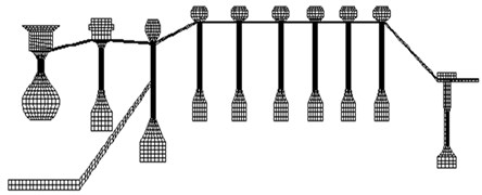
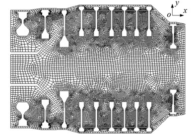
In this research, thermo-elastic coupling element Plane77 is applied to mesh the high pressure rotor. For improving the calculation accuracy, here the number of elements is 2203, and the number of nodes is 7602. Fig. 2 shows physical model of the high pressure rotor in natural convection heat transfer.
Fig. 1Cutaway view of 3D solid model
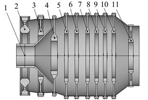
Fig. 2Finite element model of high pressure rotor
As the model is very complicated, the calculation requires plenty of time and is also difficult to converge. So, applying the symmetry of geometric model, the 2D cavity model is adopted to research natural convection heat transfer in the high-pressure rotor, as is shown in Fig. 3(a).
The cavity of high pressure rotor is meshed by flow and thermal coupling element Fluid141, and the CFD model is obtained as shown in Fig. 3(b). In the meshing process, solid wall and the region where the flow changes significantly are meshed finely. Here the number of elements is 11310, and the number of nodes is 12442.
Fig. 3Physical model of nature convection for high pressure rotor
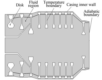
a) The two-dimensional geometric model
b) The cavity CFD model of high pressure rotor
3.2. The definition of boundary conditions
The heat exchanges between turbine disk and boundary airflow mainly include heat exchange between turbine disk surface and cooling air, heat exchange between outer edge surface and blade root, heat exchange between the outside of rotor drum and cooling air, heat transfer between the passage and cooling air. The formulas of heat transfer applied in each part are as follows:
(1) Heat exchange between turbine disk surface and cooling air.
According to the principle of convective heat transfer [31], total heat on the surface of turbine disk is expressed as:
Total heat on the surface is transmitted by conduction, so it is also expressed as:
Further processing, it can be obtained:
For making the equation dimensionless, the radius of local wheel is multiplied on both sides:
The right side of Eq. (27) is the ratio of surface temperature gradient to the reference temperature gradient. The left side is the ratio of conductive thermal resistance to fluid convection thermal resistance, and it is defined as Nusselt number . So, it is obtained:
By the empirical formula [32], the value of Nusselt number can be determined by Reynolds number . When < 2.4×10⁵, 0.675×0.5, and when > 2.4×10⁵, 0.0217×0.8:
where is thermal conductivity of cooling air, is the radius of local wheel, is circumferential speed at wheel radius , is kinematic viscosity of cooling air.
(2) Heat exchange between outer edge surface and blade root.
The heat transfer coefficient between outer edge and blade root is converted into a third type of boundary condition between outer edge and the gas. Through the convective heat transfer between the gas and blade, the heat is transferred from the blade to blade root, and then to the outer edge of turbine disk. So, the direct equivalent relationship of heat transfer is established between the gas and outer edge of turbine disk. The equivalent third type of boundary condition is:
where is the equivalent coefficient of convective heat transfer and is a function of the gas and blade parameters, is the temperature of gas, other parameters have the same meaning as before.
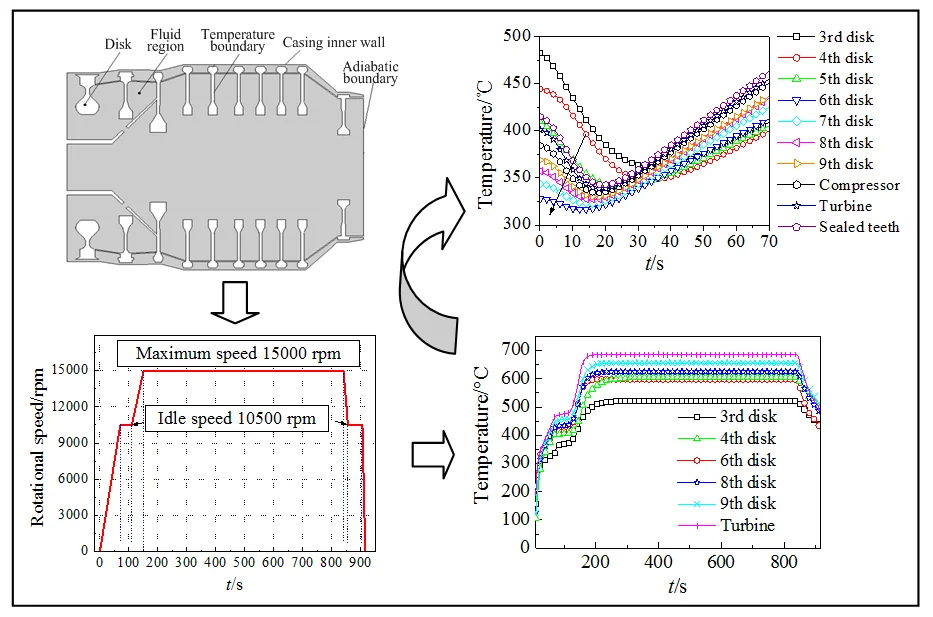
Fig. 4 shows a typical operating condition curve for aeroengine high-pressure rotor. The high pressure rotor accelerates from 0 rpm to the idle speed 10500 rpm. After a short constant speed platform, it continues to accelerate to 15000 rpm, and runs for 690 s at a constant speed of 15000 rpm. Then the rotor slows down from 15000 rpm to 0 rpm, the whole process has gone through 915 s.
Boundary conditions are changed with the engine state, while heat transfer empirical formula, calculation parameters and methods are the same in thermal boundary conditions. So, the heat transfer boundary for typical working condition can be obtained by the steady state condition, and other heat transfer boundary condition can be obtained by linear interpolation. In this research, the calculation of temperature is a pseudo-transient temperature field.
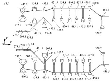
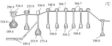
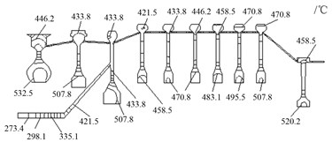
Temperature distribution of rotor outer wall at the last stop moment is taken as the initial boundary condition, as is shown in Fig. 5. The temperature of casing inner wall is constant at 20 ℃, the other solid walls are insulated. The velocity of all solid walls is assumed to be no slip, and that is 0 m/s. In the fluid region, physical properties are adopted the ideal gas parameters at 20 ℃.
4. Discussion and analysis of results
4.1. Thermal-elastic coupling characteristics at typical start and stop conditions
(1) The distribution of transient temperature at typical start and stop conditions.
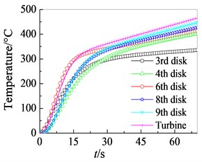
Temperature curves at typical operating conditions are obtained on different nodes, as are shown in Fig. 6.
Fig. 6(a) shows the temperature curves of different nodes in the whole process. During the process of start, the highest temperature is at outer edge of high pressure turbine. This zone exchanges heat with high temperature gas, so the temperature is higher, and is basically synchronized with the boundary temperature.
Fig. 4Speed curve during star and stop times
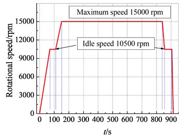
Fig. 5Boundary condition of initial temperature
When start process is completed, the highest temperature of zone reaches a stable value. The time required for temperature field to stabilize is longer than the stabilization time of heat exchange boundary condition for 150 s. The stabilization time of highest temperature is exceeded by 190 s. It also shows that the temperature rise rate and warm-up are significantly reduced in the start process. Due to the vibration of thermal bending, it usually makes the amplitude increase significantly in the process of slow speed start. So, the temperature change is given in this start period, as is shown in Fig. 6(b).
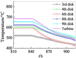
Fig. 6(c) shows the temperature curves of different nodes at the stop process. As the stopping time is short, the whole rotor has a higher temperature when the stop speed is reduced to 0 rpm. For the temperature difference of high pressure rotor, natural convective heat transfer occurs at the process of natural cooling.
Fig. 6Temperature curves of high pressure rotor at start and stop process
a) At the whole process
b) At the slow speed start process
c) At the stop process
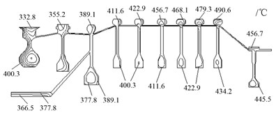
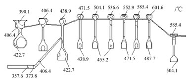
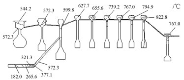
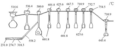
Fig. 7 shows the temperature distribution of high pressure rotor at different moments. It can be found that isoline density of the temperature at the third stage disk is larger in rotor start process, and indicates that the change of temperature is more obvious in this region. Rotor temperature increases gradually from the lower stage to the higher stage, and the temperature of outer edge in each disk is higher than the temperature of inner edge.
When start process reaches a steady state, the lowest temperature appears in the region of front section, temperature value is 357.6℃. The highest temperature appears in the outer edge at the first stage disk, the temperature value is 601.6℃, and it is shown in Fig. 7(c). Because the time of stop process is shot, temperature change isn’t shown a constant speed (10500 rpm) platform for 50 s, and cooling rate is always large. Fig. 7(f) shows the final temperature distribution at the end of whole process. It is adopted as the temperature boundary condition for flow-thermal coupling calculation in natural convective heat transfer.
Fig. 7Temperature distributions of high pressure rotor at different start moments
a) 30 s
b) 60 s
c) 130 s
d) 400 s
e) 850 s
f) 915 s
(2) Thermal-elastic coupling characteristics at start and stop process.
The calculation of stress field is taken a sequential coupling approach. Based on the distribution of temperature field, node temperature is loaded to the model of stress calculation. Then the degree of freedom is constrained, blade centrifugal force and fluid pressure of external flow field are ignored.
Transient displacements of high pressure rotor at different nodes and moments are shown in Fig. 8. It can be found that radial displacement of each node is basically in the same law, the change is significant at start and stop process. The radial displacement curves of high pressure rotor are shown in Fig. 9.
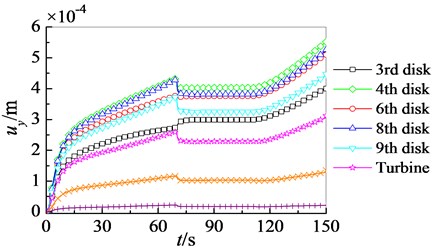
In Fig. 9(a), radial displacement of each node gradually increases with the increase of start time. When rotational speed is 10500 rpm, the value of radial displacement is decreased suddenly. It is because the coefficient of convective heat transfer at this moment is kept constant. The change of each node temperature is decreased, and the difference of temperature is gradually reduced, so the displacement is gradually decreased. Then the temperature is gradually increased with rotational speed, the difference of temperature is increased, and radial displacement is increased.
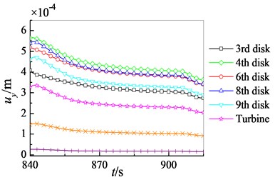
Fig. 9(b) shows the radial displacement curves of high pressure rotor at stop process. As the time of stop process is shot, radial displacement isn’t shown a constant speed 10500 rpm platform for 50 s, and is increased with stop time. This illustrates that temperature difference, thermal stress and thermal deformation are much large in stop process.
Fig. 8Transient displacement of high pressure rotor at different nodes and moments
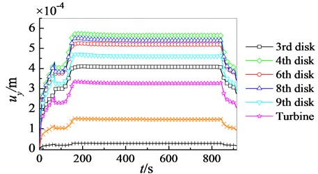
Fig. 9Radial displacement distributions of high pressure rotor at start and stop process
a) The process of start
b) The process of stop
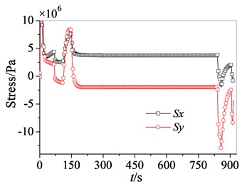
Fig. 10 shows response curves of the first stage disk on high pressure rotor. It can be found in Fig. 10(a) that the radial and axial stresses have the same law, and the larger thermal stresses are generated at the start and stop process. The maximum stress occurs at the moment when the speed is accelerated to 15000 rpm (starting time 150 s). The value of rotor stress becomes small with the stabilization of rotor temperature. Fig. 10(b) exhibits that radial displacement of the rotor is much larger than axial displacement. Total displacement is basically the same as radial displacement, and axial displacement has little effect on the total displacement. Hence, the effect of axial thermal deformation on high pressure rotor is ignored in the research of thermal vibration.
Fig. 10Response curves of the first stage disk on high pressure rotor
a) The curves of thermal stress
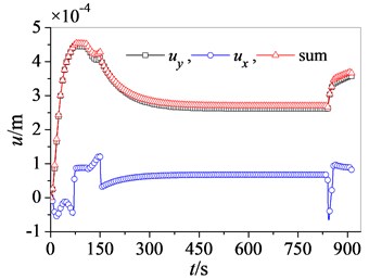
b) The curves of displacement
Fig. 11 shows displacement distributions of high pressure rotor at different moments. It reflects the change of displacement at different moments.
Fig. 11Displacement distributions of high pressure rotor at different moments
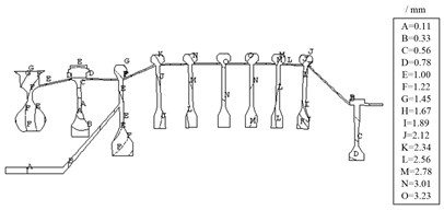
a) 30 s
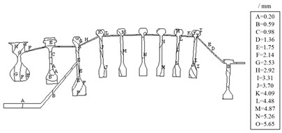
b) 160 s
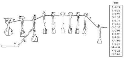
c) 600 s
d) 850 s
e) 910 s
4.2. Flow-thermal coupling characteristics of natural convection conditions after stopping
(1) Flow law of rotor cavity at stop process.
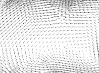
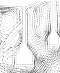
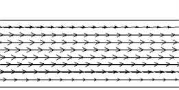
Fig. 12 shows the distribution of steady velocity contour in high pressure rotor cavity. Due to the complexity of calculating geometric model and temperature boundary condition, velocity distribution of the whole computational domain is also very complex. In particular, velocity contour of each disk cavity are distributed densely, and it changes more obviously.
Fig. 13 shows the distribution of velocity vector in rotor cavity. In Fig. 13(a), it is macroscopically exhibited the velocity vector distribution of natural convective air. As physical model of the high pressure rotor is much complex, the density of discretized grid is large. In order to more clearly understand the velocity distribution of air flow, velocity vector distributions of different typical regions are shown in Fig. 13(b).
Fig. 12Velocity contour distribution in high pressure rotor cavity
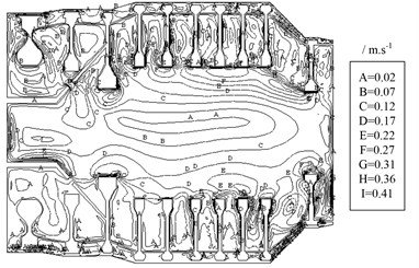
Fig. 13Velocity vector distribution in high pressure rotor cavity
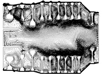
a) The diagram of macroscopic velocity vector
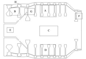
b) Sketch map of different typical regions
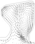
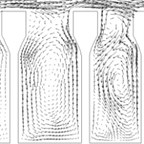
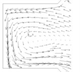
Fig. 14 shows the local magnification diagrams of velocity vector at different regions. In Fig. 14(c), a large typical ellipse vortex is formed between upper and lower surfaces. Its flow characteristic is similar to natural convection in a square cavity. But the position of large ellipse vortex is taken a certain offset, and it is located at bottom right position of the cavity.
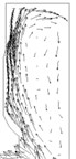
Fig. 14(a) and (d) exhibit the flow characteristics of disk cavities in the upper and lower regions. In the adjacent upper cavities formed by the 7th, 8th and 9th disks, the characteristics of air flow are basically similar, and a typical ellipse vortex is formed in the cavity. It is different in the two adjacent lower cavities, three ellipse vortexes are formed in the high temperature disk cavities. While only one ellipse vortex is formed in the low temperature region, and the flow velocity also has a significant difference.
Fig. 14(b) shows the velocity vector distributions in the cavities of 3rd disk and 4th disk. When the air flows from narrow passage, most of it flows into the cavities of 3rd disk and 4th disk, and immediately forms two vortexes in left and right sides. Only a little amount of air flows into the small gap formed by high pressure rotor and the casing.
In Fig. 14(e), a large ellipse vortex is formed in the E region, and the velocity of flow is large. Flow characteristics of other areas are not described in detail. In short, due to geometrical complexity of high pressure rotor and nonlinear variation of temperature boundary along the axial direction, natural convection of the air is very complicated in high pressure rotor cavity. Many annular vortexes are formed in the whole cavity, which is completely different from natural convection of simple square cavities. It shows the diversity and complexity of flow.
Fig. 14Local magnification diagrams of velocity vector at different regions
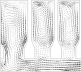
a) Region A
b) Region B
c) Region C
d) Region D
e) Region E
f) Region F
g) Region G
h) Region H
(2) Flow-thermal coupling characteristics at natural convection condition.
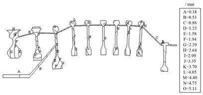
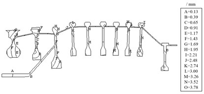
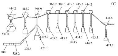
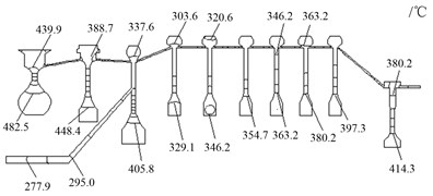
Different coefficients are selected as convective boundary conditions in each rotor part, which is obtained by the calculation of natural convection flow-thermal coupling. The distribution of thermal-elastic coupling field is analyzed at different stop moments. Fig. 15 shows the temperature distribution in rotor upper region.
At the beginning of stop, the temperature of rotor is much higher. The density of temperature contour is larger, especially at the 3rd and 4th disks. The temperature of each node gradually decreases with the increasing of stop time. The density of temperature contour decreases in the same time, it illustrates that temperature distribution of high pressure rotor gradually becomes uniform. By comparison, it is found that the reduction of temperature is relatively smaller at the 3rd and 4th disks, and the density of contour is much larger. This is mainly because the velocity of air flow is relatively small at the 3rd and 4th disks, and the coefficient of convective heat transfer is small. Hence, it makes drop amplitude of the temperature in a lower value.
Fig. 15Temperature distributions of high pressure rotor at different stopping moments
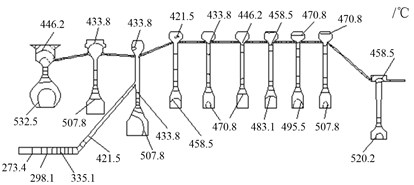
a) 0 s
b) 100 s
c) 300 s
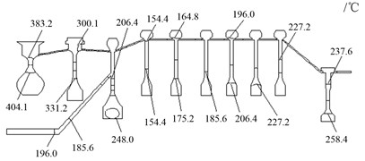
d) 1000 s
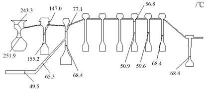
e) 3000 s
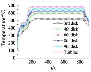
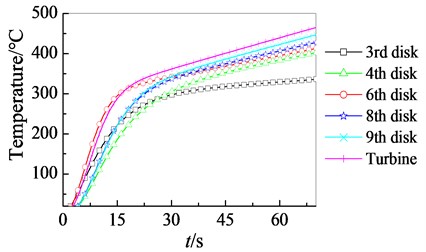
Fig. 16 shows temperature curves of different locations after stopping. The temperature of each node gradually decreases with the increase of stopping time. Cooling speed of the temperature is the slowest at the 3rd disk, while cooling speed is the fastest on the 8th disk. After stopping time reaches 90 minutes, temperature change of each node becomes much slower. Eventually the temperature of each node is equal to the temperature of room, and the heat exchange tends to be balanced.
Fig. 17 shows the curves of temperature difference between the upper and lower surfaces after stopping. The difference of temperature isn’t gradually decreased with the increase of stopping time, it presents a phenomenon of increasing firstly and then decreasing. Besides that, the maximum temperature difference of different positions appears at different moments. Here the maximum temperature difference is about 23 ℃ at the 3rd disk, and appears near 60 minutes after stopping. The minimum temperature difference is about 4.8 ℃ at the 8th disk, and appears near 15 minutes after stopping. It also can be found that temperature difference at the 3rd disk is larger in the stopping time of 40-90 min, and is more than 20 ℃. This is basically consistent with the operating experience, so the correctness of calculation is verified.
Fig. 16Temperature curves at different moments
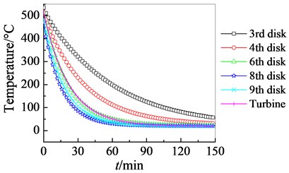
Fig. 17Difference curves of the temperature
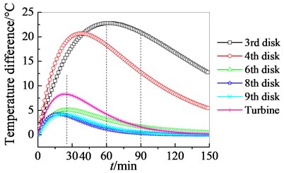
Fig. 18 shows thermal stress curves of high pressure turbine in and directions. After stopping, the cold air and hot air form a convection process in the high pressure turbine cavity. It makes the temperature difference of high pressure turbine change alternately, so thermal stress fluctuates greatly at the beginning of stopping period. The convection of cold air and hot air becomes slower with the time consumption, and temperature difference becomes small and stable. When stopping time reaches 1500 s, stress value remains basically unchanged. It illustrates that heat exchange has been completed at this moment, and temperature difference of the rotor changes little.
Fig. 18Thermal stress curves of high pressure turbine in x and y directions
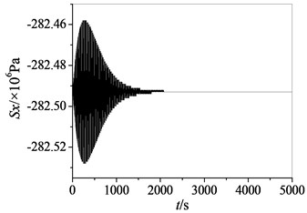
a) In the direction
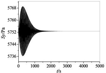
b) In the direction
Fig. 19 shows temperature curves of idle speed in restart process after stopping. The temperature of each node decreases firstly and then gradually increases in the restart process after parking 300 s, as is shown in Fig. 19(a). The time corresponding to the lowest temperature is also different in each position. Here it is the longest in the 3rd disk, and is about 35 s. While it is the shortest in the 8th disk, and is about 12 s. Except that the temperatures of the 3rd disk and 4th disk decrease firstly and then increase gradually when the parking time is increased to 1200 s in Fig. 19(b), the other nodes are gradually increased with starting time. When the stopping time is increased to 5000 s in Fig. 19(c), temperature change of each node has become balanced on high pressure turbine, and it is equal to room temperature. So, the start at this moment is equivalent to a cold start.
Fig. 20 shows difference curves of temperature in restart process at different stop moments and positions. Fig. 20(a) exhibits temperature difference of the 3rd disk gradually decreases with the time of restart after different stop moments. When start time increases to 50 s, temperature difference between the upper and lower surfaces is 0 ℃ at the 3rd disk. Fig. 20(b) exhibits temperature difference of different position in restart process after stopping 3600 s. As the start time increases, temperature difference between the upper and lower surfaces gradually decreases. Here temperature difference of the 3rd disk is the largest, and temperature difference of the 6th disk is the smallest. When the starting time is increased to 50 s, temperature difference is the smallest in each node.
Fig. 19Temperature curves of idle speed in restart process
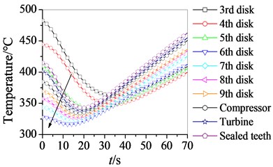
a) After stopping 300 s
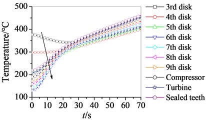
b) After stopping 1200 s
c) After stopping 5000 s
Fig. 20Difference curves of temperature in restart process
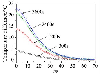
a) At the 3rd disk
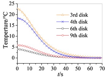
b) At different positions
5. Conclusions
Based on the typical start and stop conditions of aeroengine high pressure rotor, the problem of flow-thermo-elastic coupling is solved in this research. Applying basic theory and control equation, it is analyzed the fields of transient temperature, thermal stress and thermal deformation in the start and stop process. Then the temperature at last stopping moment is selected as the boundary condition. With the flow-thermo-elastic coupling method, the distributions of air flow, heat transfer and temperature are discussed in high pressure rotor cavity. The results show:
1) The distributions of flow field and temperature field are calculated when aeroengine high pressure rotor is stopped. At the beginning of stop period, the rotor has a higher temperature, and the density of temperature contour is much larger, especially at the 3rd and 4th disks. With the increasing of stop time, the temperature of each node gradually decreases. When stop time is within 40-90 minutes, temperature difference between the upper and lower surfaces is larger than 20 ℃. This is basically consistent with the operating experience, which verifies the correctness of calculation in this research.
2) The distribution of transient temperature is studied at natural convection heat transfer in restart process. It is different when restart process is taken at different stop moments. If the stop time is short, temperature distribution of the rotor is decreased firstly, then increased, and finally decreased. The time corresponding to the lowest temperature is also different in each node. It is the longest in the 3rd disk, and the shortest in the 8th disk.
References
-
Lu S., Zhao M., Ren P., et al. A numerical analysis of thermal bending deformation and its influence on rotor. Journal of Aerospace Power, Vol. 12, Issue 3, 1997, p. 243-246.
-
Chen L., Dugundji J. Thermal stress and gas bending effects on vibration of compressor rotor stages. Journal of Aircraft, Vol. 17, Issue 8, 2014, p. 576-583.
-
Zhuo M., Yang L., Zhang Y., et al. Analysis of rotor thermal bow and vibration response in gas turbine. Journal of Mechanical Engineering, Vol. 53, Issue 3, 2017, p. 57-62.
-
Guo X., Wu X., Jiang G. Experimental investigation of rotor vibration fault caused by rotor thermal bending. Journal of Shenyang Aerospace University, Vol. 32, Issue 5, 2015, p. 26-31.
-
Davis G. Natural convection of air in a square cavity: A bench mark numerical solution. International Journal for Numerical Methods in Fluids, Vol. 3, Issue 3, 1983, p. 249-264.
-
Barakos G., Mitsoulis E., Assimacopoulos D. Natural convection flow in a square cavity revisited: Laminar and turbulent models with wall functions. International Journal for Numerical Methods in Fluids, Vol. 18, Issue 7, 1994, p. 695-719.
-
Girgis I. Numerical and experimental investigations of natural convection in inclined air enclosures. AIAA Journal, Vol. 38, Issue 1, 2000, p. 10-13.
-
Dong S., Li Y., Liu Y. Simulation of the natural convection in a closed cavity with vortex-stream function method. Low Temperature and Specialty Gases, Vol. 21, Issue 6, 2003, p. 16-21.
-
Huang J., Li G., Jiang X. Numerical study on the flow transition in laminar natural convection flow in a square cavity. Journal of Huazhong University of Science and Technology, Vol. 29, Issue 5, 2001, p. 51-53.
-
Dong S., Li Y. Conjugate of natural convection and conduction in a complicated enclosure. International Journal of Heat and Mass Transfer, Vol. 47, Issue 10, 1983, p. 2233-2239.
-
Atmane M., Chan V., Murray D. Natural convection around a horizontal heated cylinder: The effects of vertical confinement. International Journal of Heat and Mass Transfer, Vol. 46, Issue 19, 2003, p. 3661-3672.
-
Goloviznin V., Korotkin I., Finogenov S. Modeling of turbulent natural convection in enclosed tall cavities. Journal of Applied Mechanics and Technical Physics, Vol. 58, Issue 7, 2017, p. 1211-1222.
-
Shahi M., Mahmoudi A., Talebi F. Numerical study of mixed convective cooling in a square cavity ventilated and partially heated from the below utilizing nanofluid. International Communications in Heat and Mass Transfer, Vol. 37, Issue 2, 2010, p. 201-213.
-
Xu H. Numerical simulation of unsteady natural convection from heated horizontal circular cylinders in a square enclosure. Numerical Heat Transfer Part A Applications, Vol. 65, Issue 8, 2014, p. 715-731.
-
Das M., Reddy K. Conjugate natural convection heat transfer in an inclined square cavity containing a conducting block. International Journal of Heat and Mass Transfer, Vol. 49, Issue 25, 2006, p. 4987-5000.
-
Balaji C., Venkateshan S. Combined conduction, convection and radiation in a slot. Fuel and Energy Abstracts, Vol. 36, Issue 2, 1995, p. 139-144.
-
Vynnycky M., Kimura S. Conjugate free convection due to a heated vertical plate. International Journal of Heat and Mass Transfer, Vol. 39, Issue 5, 1996, p. 1067-1080.
-
Merkin J., Pop I. Conjugate free convection on a vertical surface. International Journal of Heat and Mass Transfer, Vol. 39, Issue 7, 1996, p. 1527-1534.
-
Kimura S., Okajima A., Kiwata T. Conjugate natural convection from a vertical heated slab. International Journal of Heat and Mass Transfer, Vol. 41, Issue 21, 1998, p. 3203-3211.
-
Méndez F., Treviño C. The conjugate conduction-natural convection heat transfer along a thin vertical plate with non-uniform internal heat generation. International Journal of Heat and Mass Transfer, Vol. 43, Issue 15, 2000, p. 2739-2748.
-
Chen L., Tian H., Li Y., et al. Investigation to conjugated natural convection heat transfer from a vertical plate with discrete heat sources. Journal of Xi’an Jiaotong University, Vol. 40, Issue 9, 2006, p. 1014-1018.
-
Chen L., Tian H., Li Y., et al. The numerical research on the natural convection of vertical plate with uneven temperature distribution. Industrial Heating, Vol. 35, Issue 2, 2006, p. 20-23.
-
Kuo W., Lie Y., Hsieh Y., et al. Condensation heat transfer and pressure drop of refrigerant R-410A flow in a vertical plate heat exchanger. International Journal of Heat and Mass Transfer, Vol. 48, Issue 25, 2005, p. 5205-5220.
-
Ibrahim W., Makinde O. D. The effect of double stratification on boundary-layer flow and heat transfer of nanofluid over a vertical plate. Computers and Fluids, Vol. 86, Issue 7, 2013, p. 433-441.
-
Arquis E., Rady M. Study of natural convection heat transfer in a finned horizontal fluid layer. International Journal of Thermal Sciences, Vol. 44, Issue 1, 2005, p. 43-52.
-
Abdallah M., Zeghmati B. Natural convection heat and mass transfer in the boundary layer along a vertical cylinder with opposing buoyancies. Journal of Applied Fluid Mechanics, Vol. 4, Issue 4, 2011, p. 15-21.
-
Bondareva N. S., Sheremet M. A. Natural convection heat transfer combined with melting process in a cubical cavity under the effects of uniform inclined magnetic field and local heat source. International Journal of Heat and Mass Transfer, Vol. 108, Issue 5, 2017, p. 1057-1067.
-
Mbeledogu I., Ogulu A. Heat and mass transfer of an unsteady MHD natural convection flow of a rotating fluid past a vertical porous flat plate in the presence of radiative heat transfer. International Journal of Heat and Mass Transfer, Vol. 50, Issue 9, 2007, p. 1902-1908.
-
Sivasankaran S., Do Y., Sankar M. Effect of discrete heating on natural convection in a rectangular porous enclosure. Transport in Porous Media, Vol. 86, Issue 1, 2011, p. 261-281.
-
Kamiyo O., Angeli D., Barozzi G., et al. A comprehensive review of natural convection in triangular enclosures. Applied Mechanics Reviews, Vol. 63, Issue 6, 2010, p. 1463-1472.
-
Incropera F. P., DeWitt D. P. Fundamentals of Heat and Mass Transfer. Wiley, New York, 1996.
-
Gnielinski V. Neue Gleichungen für den Wärme-und den Stoffübergang in turbulent durchströmten Rohren und Kanälen. Forschung im Ingenieurwesen A, Vol. 41, Issue 1, 1975, p. 8-16.
About this article

The work is supported by Natural Science Foundation of Liaoning Province (Grant No. 20180550880), Education Department Series Project of Liaoning Province (Grant No. L201746) and Young Doctor Scientific Research Foundation of College (Grant No. 17YB04).
