Pavement roughness identification research in time domain based on neural network

1. Introduction

Pavement roughness has been defined as the variation in surface elevation that induces vibrations in traversing vehicles. Earlier studies [1] (Gillespie and Sayers 1983) have shown that rough roads lead to user discomfort, increased travel time due to speed reductions and higher vehicle cost [1, 2]. Besides, early roughness deterioration induces high dynamic vehicle axle loading, which might create unexpected road damage and distress deterioration. Pavement roughness provides a good, overall measure of pavement condition [3, 4]. In the process of researching vehicle’s riding comfort and handling stability, whether pavement roughness can reflects the true situation of the road plays a key role in the accuracy of vehicle performance analysis. In that case, when studying vehicle ride comfort and handling stability, how to get a reasonable pavement roughness is one of the most important issue to be solved.

When driving, pavement roughness is the main incentive. It is the key point to get accurate road information to analyze and evaluate vehicle’s riding comfort. But, early pavement research method is experimentation [5-9]. This method has advantages of visual interpretation and effectiveness, but it takes a lot of hard work and time and is diseconomy. Loading identification technology to research the pavement roughness is tried to be used in this paper. Pavement roughness is the basic input of vehicle’s vibration. Whether pavement roughness is accurate has a big impact on the study of vehicle’s ride performance and handling stability. So how to get accurate pavement roughness is need to be solved. There are two ways to identify load information: frequency domain and time domain methods. Comparing with the frequency domain method, the time domain method has many advantages. First, the time domain method is easy to analyze nonlinear feature. Second, the time domain method is able to get respondent value directly such as the maximum of velocity, force and acceleration. Third, the amplitude domain and frequency domain can be achieved according to the information of time domain. So in this paper time domain recognition method is adopted.

Back propagation (BP) neural network has disadvantages of slowly convergence speed and local minimum value. However, radial basis function (RBF) neural network is a kind of feed forward neural network with high performance. It has little calculation, better learning speed than BP neural network. It also has a stronger ability of parameter approximation and classification than BP neural network. GRNN is a special form of radial basis function neural network [10-11]. Its abilities of approximate function and learning are very strong. So this special radial basis function neural network is used in this paper to recognize pavement roughness.

2. Establishment of vehicle vibration model with 7 DOFs

When vehicles are running on an uneven road, the heights of the left and right wheel ruts are different, the longitudinal mass distribution of the left and right wheels are approximately symmetrical. In that case, it will lead to a roll movement of vehicle body. Vehicle vibration model with 7 DOFs is introduced in order to take account of the vehicle’s roll movement when studying vehicle’s riding comfort. The vertical movement, roll and pitching movement of vehicle are also considered in this 7 DOFs vehicle model.

The following assumptions are made when establishing vehicle’s dynamical model with 7 DOFs:

1) Regarding vehicle body as a rigid body with lumped mass, only vehicle body’s vertical vibration, roll movement and pitching movement are considered. The effects of twisting vibration of vehicle body on vehicle’s riding comfort is ignored.

2) Assuming the vehicle body to do micro-vibration in the vicinity of the equilibrium position and suspension stiffness and damping are treated as constants, the vehicle body is treated as a linear system to handle.

3) Vehicle is symmetrical about the vertical centerline and does uniform rectilinear motion.

4) Pavement is a steady ergodic normal random process with isotropic.

5) Other vibration sources are ignored except pavement roughness.

According to the above assumptions, the vehicle can be simplified as a spatial 7 DOFs dynamic model, as shown in Fig. 1.

Fig. 1Vehicle vibration model with 7 DOF

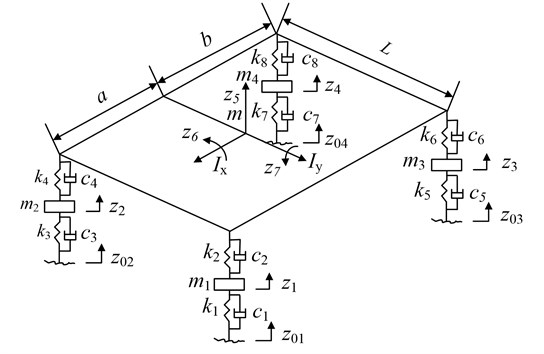
According to Lagrange’s equation, vehicle’s vibration equation can be acquired as follow:

where $\mathbf{M}$ – the mass matrix of vehicle, $\mathbf{C}$ – the damping matrix of vehicle, $\mathbf{K}$ – the rigidity matrix of vehicle, $\mathbf{Z}$ – the displacement vector of each dof of vehicle, $\mathbf{Q}$ – the vector of pavement input, ${\mathbf{K}}_t$ – the rigidity matrix of tires, ${\mathbf{C}}_t$ – the damping matrix of tires.

The above formula and the meaning of each of the parameters in Fig. 1 are explained in Appendix.

3. Pavement input function of four-wheel vehicle

It is proved by practice that the right wheels and the left wheels have spatial correlations.

Assuming wheel rut $x$ has a white noise input $W_x$ and the other wheel rut $y$ has a white noise input $W_y$, the relationship between the two wheel ruts are established. Then the incentive elevation input of each front and back point of $y$ traces is calculated. According to the random vibration theory of linear system, when the process of input is smooth, so will be the output process. In this case, the problem can be simplified as follows: input of a wheel rut, then determine the output of other wheel rut and establish the relationship between input and output with the coherence function ${\mathrm{c}\mathrm{o}\mathrm{h}}_{xy}\left(f\right)$. In other words, the relationship of transmission between right and left wheel ruts is established and a wheel rut’s random process can be deduced from the other wheel rut’s. Using front wheel as a reference point, assuming transfer function of road surface white noise input between right and left wheels $W_x$, $W_y$ is:

The following equation is obtained by using second order approximate solution:

The coefficients in the function are got by fitting and converting coherence functions which measured from different pavements.

With the intermediate variable $M\left(s\right)$, the above equation turns into:

Further, the Eqs. (5), (6) was obained by converting numerator and denominator of Eq. (4):

Seting state variables $x_1=L^{-1}\left(s^{-1}M\right(s\left)\right)$, $x_2=L^{-1}\left(s^{-2}M\right(s\left)\right)$.

Because $L\left[{\dot{x}}_2\right]=sL\left[x_2\right]=s{s}^{-2}M\left(s\right)=s^{-1}M\left(s\right)=L\left[x_1\right]$, then ${\dot{x}}_2=x_1$.

By using inverse Laplace transform and combining the result with ${\dot{x}}_2=x_1$, the correlation state equation is obtained from Eq. (5):

Similarly, the output $W_y$ equation is obtained by using the inverse Laplace transform of Eq. (6):

The ${\dot{x}}_1$ determined by the equation from Eq. (7) is substituted into Eq. (8), $W_y$ is calculated as follows:

When $W_x$ generates one wheel rut, the white noise input $W_y$ is obtained from Eq. (8) by the intermediate state variable $x_1$ and $x_2$ from Eq. (7). Then the space-related time-domain model between the second wheel rut and the first wheel rut is obtained as:

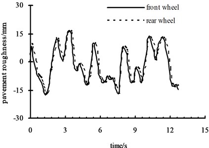
Assuming the average phase difference of incentives between two wheel cuts is zero. Using the coherence function method and according to module of frequency response function and the formula of coherence function $H\left(\omega \right)=\mathrm{c}\mathrm{o}\mathrm{h}\left(\omega \right)$, the coefficients of Eq. (3) is got: $a_0=$ 3.1815, $a_1=$ 0.2063, $a_2=$ 0.0108, $b_0=$3.223, $b_1=$ 0.59, $b_2=$ 0.0327. The roughness incentives of four-wheel vehicle on C-level road are shown in Fig. 2 and Fig. 3 by programming and simulating with Matlab.

Fig. 2Pavement roughness of left front and rear wheels

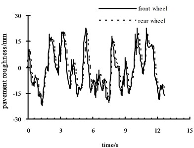
Fig. 3Pavement roughness of right front and rear wheels

4. Generalized regression neural network structure

Generalized regression neural network (GRNN) is a special form of the radial basis neural network. GRNN has a good performance in function approximation and learning ability. So it is used in this paper. Its topological structure has been shown in Fig. 4.

Fig. 4GRNN structure figure

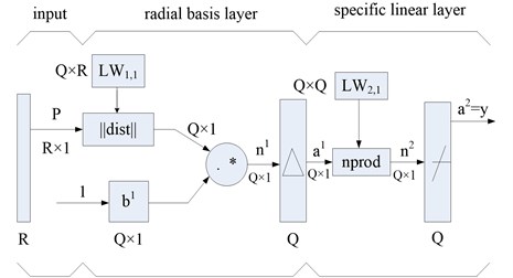
The neurons of first layer in GRNN has the same functions with the fundamental radial basis neurons. The difference between them is the special linear layer. The output of radial basis layer is computed with weight matrices $L{W}_{\mathrm{2,1}}$ by using nprod calculation method. Then the result is sent to linear transfer function. The above processes could be accomplished with neural network toolbox in Matlab.

The number of radial basis and special linear neurons in GRNN is the same as the input sample vector. The weight matrix $L{W}_{\mathrm{2,1}}$ is set as the output vector $T$. So, if the input of real network is 1, the objective output is much closer to the network output vector $T$. Therefore, the ability of function approximation of GRNN is better than basic radial basis neural network in general problems.

Because of the application of vehicle vibration isolate system, the response of vehicle to displacement and acceleration of certain time domain pavement incentives is small. The effect of these frequency components can be ignored. Assuming the upper limit and floor limit of needed pavement time frequency components are $f_u$ and $f_l$ respectively [12]. Then the following equation can be obtained:

In this paper, the vertical acceleration and the pitching angle acceleration of the vehicle mass center are used as the ideal input sample, the corresponding pavement roughness is used as the ideal network output sample. After network training is finished, the nonlinear mapping relationship among the vertical acceleration, the pitching angle acceleration and the pavement roughness is built. The model of pavement roughness recognition has been built.

5. The simulation example

The data of a certain micro-car’s are used to do simulation calculation according to the 7 DOFs vehicle model as shown in Fig. 1. The basic data are: $m=\mathrm{}$920 kg, $I_y=$948 kg∙m², $I_x=\mathrm{}$239 kg∙m², $a=$1.109 m, $m_1=m_2=m_3=m_4=$25 kg, $L=$1.22 m, $u=$80 km/h, $b=$1.09 m, $c_1=c_3=c_5=c_7=\text{40 N∙s/m,}$$c_6=c_8=\text{3340 N∙s/m,}$$k_2=k_4=\text{16.7 kN/m,}$$k_6=k_8=\mathrm{}$21.1 kN/m, $c_2=c_4=\mathrm{}$2845 N∙s/m, $k_1=k_3=k_5=k_7=\mathrm{}$147 kN/m.

The pavement roughness of $c$-level road is simulated with Matlab. The simulation result of vehicle body centroid vertical acceleration and pitching angular acceleration on $c$-level road are shown in Fig. 5 and Fig. 6. Take the results into trained network to calculate.

Fig. 5Vertical acceleration curve

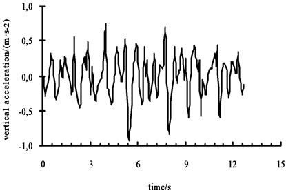
Fig. 6Pitching angular acceleration curve

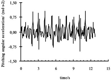
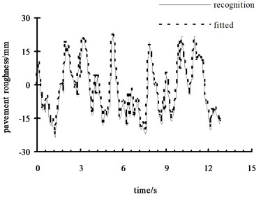
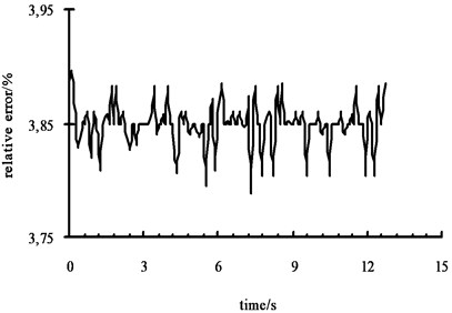
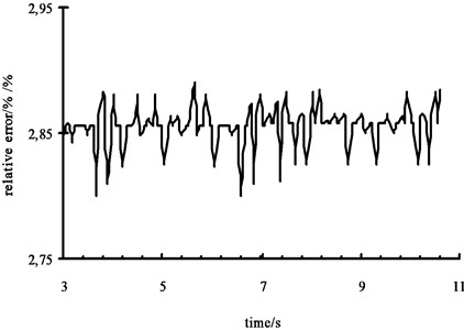
Fig. 7(a) shows the left front wheel receive the results of pavement excitation which is GRNN network recognition value in the c-level pavement by the front left wheel road excitation. Fig. 7(b) shows the relative error between recognition value and fitted value. As shown in the figure, the simulation value and recognition value agree well. It shows that the 7 DOFs model has a high precision and can describe vehicle’s actual motion well. Fig. 7(c) and Fig. 7(d) are the simulation results with noise. It shows that GRNN has a strong ability of resisting noises and high accuracy of recognition.

Fig. 7Road simulation results

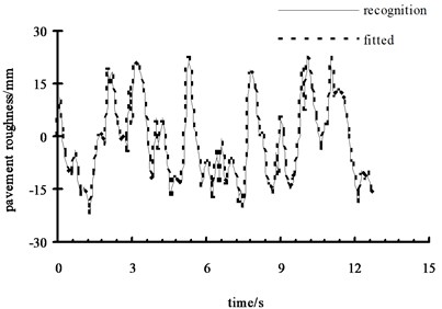
a) Recognition value and fitted value of pavement roughness

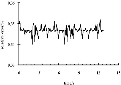
b) Relative error of pavement roughness

c) Recognition value and fitted value (with noise)

d) Relative error (with noise)

6. Building whole vehicle model by ADAMS/View

The whole vehicle model includes: vehicle body model, double arm front independent suspension model, steering mechanism model, slanting cantilever back suspension model, tire model and pavement model [13, 14]. In this paper, how to build pavement model is introduced.

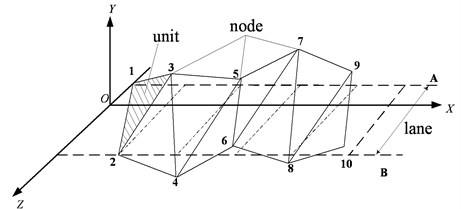
In ADAMS, the pavement is a 3D surface composed by a series of triangle elements. Triangle element is composed by a series of node and the $X$, $Y$-coordinates of those nodes need to meet certain rules. The $Z$-coordinate represents only the width of the road. Firstly, those nodes are combined to form pavement elements according to certain rules. The static frictional coefficient and dynamic frictional coefficient are set in the pavement unit. Then ADAMS can simulate a real pavement. Random pavement generation principle is shown in Fig. 8.

Fig. 8Random pavement generation principle figure

According to the harmony superposition method of pavement roughness, the process of pavement model is worked out by using VB. The process is shown in Fig. 9.

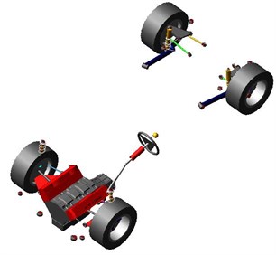
According to the corresponding constraint condition, the whole vehicle model is built by combining vehicle body model, double arm front independent suspension model, steering mechanism model, slanting cantilever back suspension model, tire model and pavement model together. The vehicle model is shown in Fig. 10.

Fig. 9Random pavement generation process figure

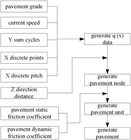
Fig. 10Vehicle model

The random pavement model is established in the vehicle model by selecting pavement generation software. Simulation time and steps are set in ADAMS software. Let the vehicle drive at 60 km/h constant speed. When the car simulation period were c-level random on the road, the measured vibration corresponding body vertical acceleration and pitch angular acceleration are used as the neural network training samples. Another group vehicle body centroid vertical acceleration and pitching angular acceleration in the c-class pavement is substituted into the already trained network and calculated by using ADAMS. As shown in Fig. 11 and Fig. 12.

The recognition value and virtual experimental value are shown in Fig. 13. The relative error of recognition value is shown in Fig. 14. It is obvious that the recognition value and virtual experimental value has a small difference. So the validity and correctness of pavement roughness recognition of GRNN is verified.

Fig. 11Vertical acceleration curve

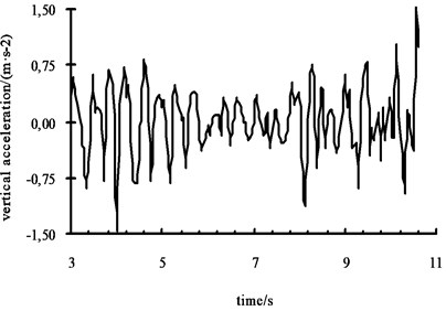
Fig. 12Pitching angular acceleration curve

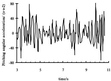
Fig. 13The results comparison figure

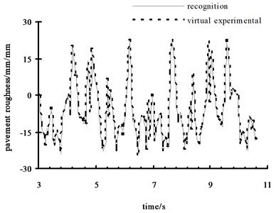
Fig. 14Relative error

7. Conclusions

On the basis of 7 DOFs vehicle model the mapping model among the vehicle body centroid vertical acceleration, pitching angular acceleration, pavement roughness is established by using GRNN. Then, another group vehicle body vertical acceleration and pitching angular acceleration is substituted into the already trained network to recognize pavement roughness. Finally, vehicle body centroid vertical acceleration and pitching angular acceleration are obtained from ADAMS virtual experiment to recognize pavement roughness. The main conclusions are as follows:

1) GRNN has a high accuracy of recognizing pavement roughness and a strong anti-noise ability. The recognized pavement roughness with noise agrees with fitted pavement roughness well.

2) The relative error between the pavement roughness recognition value and virtual experimental value is small. The correctness of using GRNN to recognize pavement roughness is validated.

3) The recognized pavement roughness provides a good foundation for the further research on vehicle’s riding comfort and handling stability.