Abstract
In this paper, off-road path recognition and navigation control method are studied to realize intelligent vehicle autonomous driving in unstructured environment. Firstly, the traversable path is achieved by vision and laser sensors. The vehicle steering and driving coupled dynamic model is established. Secondly, a coordinated controller for steering and driving is proposed via the back-stepping variable structure control method, which can be used to deal with the unmatched uncertainties of the control system model. To reduce the chattering phenomenon caused by variable structure, the boundary layer approach is introduced. The results of simulation and off-road experiment show the effectiveness and robustness of the proposed controller.
1. Introduction
Off-road intelligent vehicle has wide applications in the fields of military, civilian and planetary exploration. But the traversable off-road path is tortuous and undulates roughly without obvious marking. As a result, effectively path detection and tracking control become a challenging problem for off-road intelligent vehicle autonomous navigation.
For unstructured road detection field, the traversable path can be extracted by road features based method [1], road model based method [2] and learning based method [3] etc. Influenced by complex off-road environment and varying illumination conditions, fully reliable traversable path recognition cannot be achieved only depending on visual sensors.
Most research about tracking control of intelligent vehicle has focused on either pure longitudinal or pure lateral control [4-8]. For example, the longitudinal PI control method was extensively used for vehicle cruise control. Besides, the longitudinal controller can be designed based on the Lyapunov stability theory [9], or fuzzy-sliding mode control [10]. As for lateral controller design, basically using input-output feedback linearization [11], fuzzy theory [12-14], optimal control [15-16] and sliding-mode theory [17] based on preview model. In fact, there's tight coupling between the steering and driving dynamics of intelligent vehicle, and the coupling effects become increasingly significant especially in the off-road environment. As a result, to combine the longitudinal and lateral motion of off-road intelligent vehicle altogether, with parametric uncertainties, uncertain nonlinearities and external disturbances be concerned, a variable structure control approach based on backstepping is utilized in the paper. Besides, the chattering problem of variable structure is solved by introduce a saturation function.
2. Off-road path recognition
To realize navigation control of off-road intelligent vehicle, the desired path information need to be achieved real-time, from which the orientation deviation and lateral deviation from the preview point can be extracted. With the visual sensor and the assistant of laser sensor, the off-road path recognition is achieved and from which the desired path is extracted in the paper. The algorithm flow is shown in Fig. 1, the specific implementation steps are shown as follows:
1) Environmental information collection: the road image in front of the intelligent vehicle can be achieved through the color camera. In order to improve the reliability of the traveling regional discrimination, the convex obstacles in the road are detected based on the laser sensors. Through the pre-calibration, the correspondence relation between the laser data points and the image pixels is established.
2) Image preprocessing: The illumination compensation is made for the collected images to weaken the influence of illumination firstly. Then, the images are enhanced by histogram equalization to extract the road features. Finally, the convex obstacles region is marked to ensure that the seed points of the region-growing algorithm are selected automatically in the non-barrier region.
Fig. 1Off-road path recognition flow chart
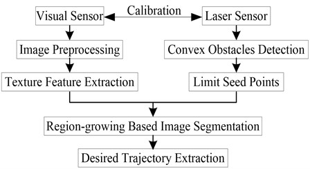
3) Texture feature extraction: As the texture can reflect the nature of image grey and the spatial relationship, the texture vector of the off-road image pixels is generated using the symbiosis matrix in this paper. The symbiosis matrix can reflect the summarized information of the image grey distribution on the direction, local neighborhood and the range of variation.
4) Region-growing based image segmentation: With the assistant of laser sensors, a traversable region near the front of the intelligent vehicle can be determined in the image. The region is taken as the road region, from which the seed points can be selected randomly. Region-growing can be conducted according to the similarity of texture and grey. Then the edges of road can be detected.
5) The extraction of desired trajectory: Morphological filter is applied for the segmented image firstly, after fill the cavity, filter the outlier, extract the Canny edge, then search the edge chain code from the image centre line to the image left and right side, get the length and the area information of the chain code, complete the left and right road edge identification. Finally, the road edge can be fitted and described by quadratic curves.
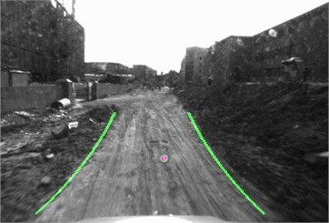
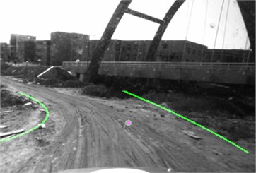
Fig. 2 shows some results of off-road path edge recognition. The right edge is taken as the desired trajectory that the intelligent vehicle needs to track in this paper, which provides the reliable and stable error feedback for the implementation of trajectory tracking control based on the vehicle preview kinematics and the driving dynamics.
Fig. 2Some off-road path recognition results
3. Vehicle dynamics
Vehicle dynamics is a nonlinear dynamics system in presence of parametric uncertainties and strong coupling characteristics. The simplified model is derived under the following assumptions: 1) Neglect roll, pitch and vertical motion; 2) Discount the brake, throttle and steering dynamics; 3) Ignore the effect of suspension on the tire axles, and approximate the tire model as linearity. The resulting equations of the simplified vehicle model are:
where , and denote longitudinal velocity, lateral velocity, and yaw angle within a fixed inertial frame, respectively. is total mass of the vehicle. is total vehicle inertia about vertical axis at center of gravity (CG). and are the distance of the front and rear axles from the CG, respectively. and are longitudinal and lateral air resistance coefficients, respectively. is rolling resistance coefficient. and are cornering stiffness of the front and rear tires, respectively. denotes the road grade, denotes gravitational acceleration (m/s2). is the steady-state engine map, denotes front wheel steering angle. denotes engine torque, is the final driver ratio, denotes transmission coefficient, denotes vehicle radius, denotes automatic transmission gear ratio, denotes engine speed, denotes throttle (%); , and denote uncertainties caused by unmodeled dynamics and time-varying parameters.
The model can be rewritten in canonical form:
where:
Assumption 1. The uncertain terms in dynamic model Eq. (1) are bounded, and there exists known continuous functions , (1, 2, 3) which satisfy following conditions:
The basic principle of longitudinal control is to make the vehicle achieve expected speed/acceleration smoothly by adjusting the driving/braking torque according to control strategic.
Given a desired velocity , actual velocity , tracking velocity error is defined as and the time derivative of is obtained as:
where is the speed error rate, and are the actual acceleration and expected acceleration, respectively. The principle of lateral control is to make intelligent vehicles accurately track the reference road. Orientation error is defined as the angle between the vehicle centerline and reference road tangent at a specified look-ahead distance , given by:
where is the orientation error at look-ahead distance , is the road curvature.
Lateral error is the horizontal distance between the vehicle position and reference road at look-ahead distance, it can be described as:
where is the lateral error at a look-ahead distance.
Intelligent vehicles control system can be yielded by combining Eq. (2), Eq. (4), Eq. (5) and Eq. (6), and control system consisting of six state variables as , , , , , and two control input variables as , , which has strict parameters state-feedback form.
4. Controller design
The lateral and longitudinal motion will be controlled when intelligent vehicles are driving, the target of lateral control is to make intelligent vehicle track the reference road, and the target of longitudinal control is to make speed errorasymptotically converge to zero. As a result, variable structure control based on backstepping is utilized to guarantee globally uniformly ultimately bounded or global asymptotic stability of tracking errors.
Coordinated longitudinal and lateral control algorithm is designed as follows.
Step 1: Considering the lateral motion, the first error vector is defined as . Choosing Lyapunov function as , and the time derivative of is obtained as:
By setting as virtual control input, the condition for tends to zero is that must be negative definite such that , where is a positive constant. Then the desired virtual control can be obtained as . Defining the difference between the virtual control input and its desired value to be the second error variable , given by:
Substituting Eq. (8) to Eq. (7) yields:
Obviously when , is satisfied. The target of next step is to search the control input variables and which can make converge to zero or a small value. Thus, is guaranteed to converge to zero or be uniformly ultimately bounded.
Step 2: Choosing Lyapunov function as and its time derivative can be obtained as:
Let:
Substituting the time derivative of Eq. (8) to Eq. (11) yields:
Substituting , , , to Eq. (12) yields:
We can get , where is positive constant, is the uncertain term that caused by the time derivative of . According to the assumption 1, there exists known continuous positive function , which satisfies .
Step 3: Considering the longitudinal motion, the error vector is defined as . Choosing Lyapunov function as , and . The condition for tends towards zero is that must be negative definite such that .
Let , where is a positive constant, is the uncertain term which caused by the time derivative of . is the time derivative of . According to the assumption 1, there exists known continuous positive function , which satisfies .
Then, an equivalent control is obtained as:
where is equivalent engine torque, is equivalent front wheel steering angle. With:
where are nonlinear damping terms, which are designed to compensate for the disturbance of uncertain terms . and are positive constant, respectively.
Choosing variable structure control law using bounded layer approach as:
where:
is saturation function. and denote thickness of boundary layer. and are positive constant, respectively.
Consequently, coordinated longitudinal and lateral control law can be expressed as:
and are the desire engine torque and front wheel steering angle, respectively. According to we can get:
The denotes desired throttle (%). From Eq. (16), is obtained as:
and satisfy the following equation:
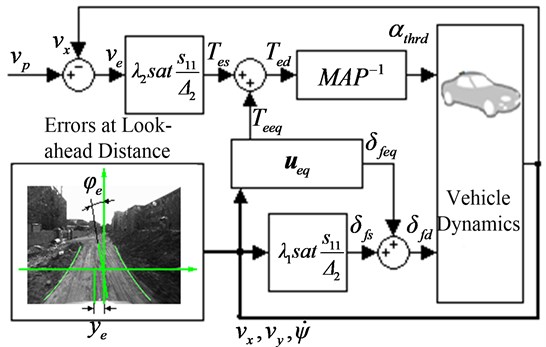
Then, the graphical diagram of the controller design is given in Fig. 3.
Fig. 3Graphical diagram of the controller
5. Stability analysis
To investigate the stability of the proposed controller, the time derivative of Eq. (8) is substituted to Eq. (10) yields:
Let , . Substituting Eq. (19) to Eq. (20) yields:
Due to , we use the method of balance for , then can get:
Let , , the final equation is obtained as:
We can get , it can be proved that error vector is uniformly ultimately bounded. Similarly, the error vector is uniformly ultimately bounded.
6. Simulation and experiment
To examine the performance of proposed control algorithms, numerical simulation tests and experiment were performed. Fig. 4 shows the experimental prototype and test environment, and the test road has changing slope and curvature, with the main features of off-road environment. Table 1 shows the main parameters of the vehicle.
Fig. 4Experimental platform
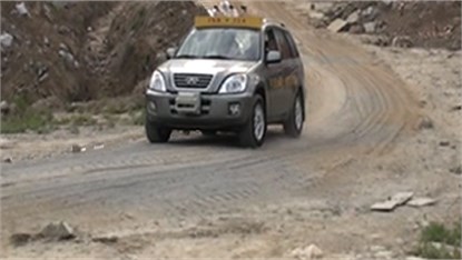
Table 1Main vehicle parameters
Parameters | Nominal value |
2100 kg | |
3059 kg·m2 | |
1.1 m | |
1.4 m | |
3.86 | |
, | 37500 Kn/rad |
0.99 | |
0.33 m | |
0.02 | |
0.79 |
The road curvature, desired velocity and acceleration profile used in simulation test are shown in Fig. 5, respectively. The initial lateral error is 0.1m, the initial orientation error is 0.02 rad, and the initial velocity error is 0.5 m/s. Fig. 6 shows the simulation results of backstepping variable structure, Fig. 6(a) is the response curve of lateral error, Fig. 6(b) is the response curve of velocity error, Fig. 6(a) and Fig. 6(b) show that lateral error and longitudinal error all can asymptotically converges to zero when the road curvature and traction acceleration change, and the controller has a strong capability of anti-disturbance and excellent robustness. Fig. 6(c) is the response curve of orientation error, and orientation error can asymptotically converge to zero when road curvature is zero. The steady-state error of orientation error larger when road curvature becomes larger, but orientation errors converged to acceptable bounds.
Fig. 5Road curvature and desired velocity
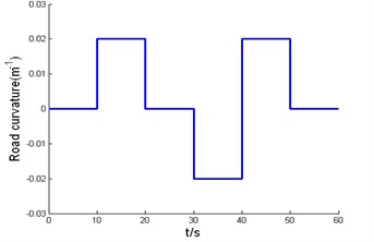
a) Road curvature
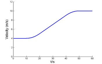
b) Expected velocity
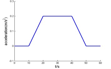
c) Expected acceleration
To demonstrate the advantages of the proposed controller, the traditional longitudinal PI controller and lateral optimal controller have been designed for comparison under the same road curvature, desired velocity and acceleration profile in Fig. 5. Firstly, the control parameter of PI controller was adjusted to make the velocity error reach the same adjustment time and control accuracy in Fig. 6(b); then, the weighting coefficient of the optimal controller to make the lateral error reach the same control level in Fig. 6(a), and the corresponding orientation error is shown in Fig. 7. It can be seen that there are significant rises in orientation error and overshoot which may lead the frequent chattering problem of steering wheel and reduce the riding comfort in the vehicle’s navigation. By contrast, as the algorithm proposed in this paper introduced a saturation function in the variable structure control, the lateral control of the vehicle is softer and the chattering problem is solved.
Fig. 6Simulation results of backstepping variable structure controller
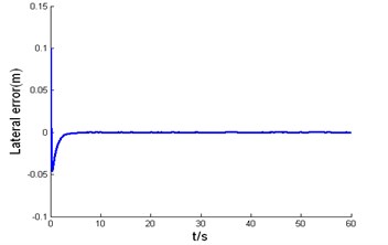
a) The response curve of lateral error
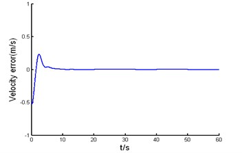
b) The response curve of velocity error
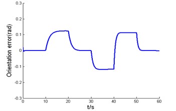
c) The response curve of orientation error
Fig. 7The response curve of orientation error under the traditional longitudinal PI controller and lateral optimal controller
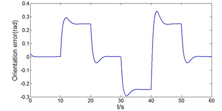
Fig. 8 shows the experimental results of the proposed controller in this paper, expected velocity is 15 km/h, The test road is rugged and includes not only the change with slope and curvature of the path, but also a certain sensor measurement error and noise, Fig. 6 demonstrate that proposed controller have good performance in the off-road environment.
7. Conclusion
The paper has presented the coupled steering and driving dynamics for off-road intelligent vehicle, and a back-stepping variable structure controller has been designed. Both simulation and experimental tests have been carried out and the results have been given. These results indicate that the proposed control strategy achieve good command tracking performance in the off-road environment.
Fig. 8Experimental results of back-stepping variable structure controller
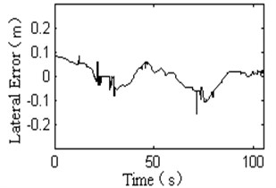
a) The response curve of lateral error
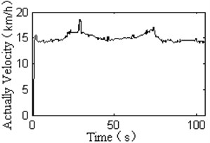
b) The response curve of velocity
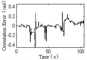
c) The response curve of orientation error
References
-
Moghadam P., Starzyk J. A., Wijesoma W. S. Fast vanishing-point detection in unstructured environments. IEEE Transactions on Image Processing, 2012, Vol. 21, Issue 1, p. 425-430.
-
Cheng H.-Y. , Yu C.-C. , Tseng C.-C., et al. Environment classification and hierarchical lane detection for structured and unstructured roads. Computer Vision, IET, 2010, Vol. 4, Issue 1, p. 37-49.
-
Milanés V., Perez J., Onieva E., Gonzalez C., et al. Lateral power controller for unmanned vehicles. Przeglad Elektrotechniczny, Vol. 86, Issue 1, 2010, p. 207-211.
-
Onieva E., Naranjo J. E., Milanes V., et al. Automatic lateral control for unmanned vehicles via genetic algorithms. Applied Soft Computing, Vol. 11, Issue 1, 2010, p. 1303-1309.
-
Onieva E., Milanes V. Vehicle Lateral Fuzzy Control Estimation. Revista Iberoamericana de Automatica e Informatica Industrial, Vol. 7, Issue 2, 2010, p. 90-92.
-
Peng Y. F. Adaptive intelligent backstepping longitudinal control of vehicleplatoons using output recurrent cerebellar model articulation controller. Expert Systems with Applications, Vol. 37, Issue 3, 2010, p. 2016-2027.
-
Chiang H. H., Wu S. J., Perng J. W., et al. The human-in-the-loop design approach to the longitudinal automation system for an intelligent vehicle. IEEE Transactions on Systems, Man and Cybernetics, Part A: Systems and Humans, Vol. 40, Issue 4, 2010, p. 708-720.
-
Guo Chunzhao, Mita S., McAllester D. Robust road detection and tracking in challenging scenarios based on Markov random fields with unsupervised learning. IEEE Transactions on Intelligent Transportation Systems, Vol.13, Issue 2, 2012, p. 1338-1354.
-
Widyotriatmo Augie, Hong Keum-Shik, Prayudhi Lafin H. Robust stabilization of a wheeled vehicle: Hybrid feedback control designand experimental validation. Journal of Mechanical Science and Technology, Vol. 24, Issue 2, 2010, p. 513-520.
-
Nasri A., Hazzab A., Bousserhane I. K., Hadjeri S., Sicard P. Fuzzy-sliding modespeed control for two wheels electric vehicledrive. Journal of Electrical Engineering and Technology, Vol. 4, Issue 4, 2009, p. 499-509.
-
Ju Yong Choi Robust controller for anautonomous vehicle with look-ahead and look-down information. Journal of Mechanical Science and Technology, Vol. 25, Issue 10, 2011, p. 2467-2474.
-
Ghaffari A., Oreh S. H. T., Kazemi R., et al. An intelligent approach to the lateral forces usage in controlling the vehicle yaw rate. Asian Journal of Control, Vol. 13, Issue 2, 2011, p. 213-231.
-
Tsai Ching-Chih, Hsieh Shih-Min, Chen Chien-Tzu Fuzzy longitudinal controller design and experimentation for adaptive cruisecontrol and Stop&Go. Journal of Intelligent and Robotic Systems, Vol. 59, Issue 2, 2010, p. 167-189.
-
Song J. Integrated control of brake pressure and rear-wheel steering to improve lateral stability with fuzzy logic. International Journal of Automotive Technology, Vol. 13, Issue 4, 2012, p. 563-570.
-
Yang D., Jacobson B., Jonasson M., Gordon T. J. Minimizing vehicle post impact path lateral deviation using optimized braking and steering sequences. International Journal of Automotive Technology, Vol. 15, Issue 1, 2014, p. 7-17.
-
Hsu Ling-Yuan, Chen Tsung-Lin An optimal wheel torque distribution controller for automated vehicle trajectory following. IEEE Transactions on Vehicular Technology, Vol. 62, Issue 6, 2013, p. 2430-2440.
-
Becerra H. M., López-Nicolás G., Sagués C. A sliding-mode-control law for mobile robots based on epipolar visual servoing from three views. IEEE Transactions on Robotics, Vol. 27, Issue 1, 2011, p. 175-183.
About this article

This project is supported by the National Natural Science Foundation of China (Grant Nos. 61203171, 61473057), China Postdoctoral Science Foundation (Grant Nos. 2012M511139, 2013T60278) and the China Fundamental Research Funds for the Central Universities (Grant Nos. DUT15LK13).
