Abstract
When a vehicle is braking or turning, the longitudinal or lateral tire forces increase greatly and it is necessary to consider the effects of vertical, longitudinal and lateral tire forces on vehicle and road dynamics. This work aims to propose a three-directional coupled vehicle-road system for revealing the properties of three-directional (3D) interaction between vehicle and road. A 23-DOF full-body heavy vehicle model considering the nonlinearity of suspension damping and tire stiffness is built, and a double-layer rectangular thin plate on viscoelastic foundation with four simply supported boundaries is employed to model the road. The equations of motion of vehicle and road, and the 3D tire forces connecting the vehicle and road are formulated. The responses of 3D coupled, vertical coupled and uncoupled vehicle-road model are compared in four maneuver conditions and the effects of parameters on 3D vehicle-road interaction are discussed. It is found that both the 3D coupled model and the vertical coupled model are good enough to predict vehicle responses accurately, but the 3D coupled model is the most suitable for calculating road responses accurately. During the maneuver of sharp steering or emergency braking, or when a vehicle runs on a road with small surface roughness and big adhesion coefficient, the role of 3D vehicle-road interaction becomes too important to be neglected.
1. Introduction
With the increase in road traffic and vehicle loads, premature damage of the asphalt pavement on expressways has become more prevalent, which has been greatly reducing the pavement’s effective lifetime. In China, some road damage occurs within the first 2 or 3 years after the road use [1]. Road damage is seen to cause an increase in dynamic tire forces, which may worsen vehicle vibration and reduce the passenger’s ride comfort and safety. Accordingly, the increased vehicle vibration leads to an increased tire force, which may speed up road damage. Hence, the vehicle and road together form a coupled system and the dynamics of vehicle and road should be investigated simultaneously based on a vehicle-road coupled system.
However, vehicle dynamics and road dynamics are two separate subjects at present. In these two subjects, the vehicle-road interaction is investigated using different models and methods, and a lot of evaluation index of road damage and design rules of vehicle and road parameters have been proposed and concluded.
In vehicle dynamics, road surface roughness is generally regarded as excitation to vehicle, and the dynamic tire loads and the road-friendly characteristics of vehicles are investigated according to road damage evaluation criterions. The popular vehicle models used for researching road-friendly characteristics includes a quarter-vehicle model with 2-DOF, a half-vehicle model with 4- or 5-DOF, a full-vehicle model with many degrees of freedom (DOF) and a Functional Virtual Prototyping (FVP) model. The dynamic load coefficient (DLC) is one of the most widely adopted evaluation criterion for dynamic interaction [2, 3]. Cole and Cebon put forward a fourth power aggregate force to evaluate the road damage induced by tire dynamic forces, which is another popular criterion for road damage. They investigated the effect of heavy vehicle parameters on tire pressure and road damage and optimized the suspension [3, 4]. Markow and Myers investigated the influence of heavy vehicle characteristics on tire forces and pavement response. They found that the vehicle configuration and suspension system greatly influences tire forces and that the tire pressure has little effect on the dynamic load [5, 6]. Sun optimized a 3-DOF quarter-truck suspension system by minimizing the dynamic pavement load and found that a large tire pressure and a small suspension damping may increase dynamic tire forces [7]. Lu validated a FVP full-vehicle model with experimental data of a heavy vehicle and discussed the effects of vehicle speed, vehicle load and road surface roughness on tire forces and DLC [8]. Chen simulated the influences of semi-active MSD and PID control on a heavy truck’s road friendliness and ride comfort through co-simulations with Adams and MATLAB [9]. It should be noted that these investigations in the field of vehicle dynamics generally assumed that the pavement was rigid and stationary and did not take into account the effect of pavement vibration on vehicle response.
In road dynamics, vehicles are generally regarded as moving loads acting on the pavement, and roads are modeled as a beam, a plate, or a multi-layer system on an elastic or viscoelastic foundation. The road response such as stress, strain and displacements of the pavement and foundation are studied analytically or numerically. And the road fatigue lifetime is predicted using different evaluation criterions, including the tensile strain at the bottom of an asphalt surface and the compressive strain in soil foundation. The Strategic Highway Research Program (SHRP) in the U.S. performed comprehensive research on road dynamics and road damage potential of dynamic wheel loads [10-11]. Hardy used the mode-superposition theory and the integral transform to derive an analytical solution of the displacement of a beam on a viscoelastic foundation, and validated it by field experiments [12]. Deng investigated the dynamics of a beam on a Winkler or a Kelvin foundation under moving vehicle loads using an integral transform [13]. Using the mode superposition and the integral transform methods, Kim studied the response of a plate on a Winkler foundation under moving loads of varying amplitude. He analyzed the influence of wheel space and driving speed on the plate displacement and stress [14]. Jeongho modeled the base and subgrade layers as stress-dependent cross-anisotropic materials and assess the pavement response using finite-element (FE) analysis. He established equations correlating the critical strains to layer displacements, axle loading, offset distance, and layer moduli in order to evaluate the accelerated damage potential due to overweight truck loading [15]. Hryniewicz presented a new analytical solution for the dynamic response of an infinitely long Timoshenko beam resting on a nonlinear viscoelastic foundation using the wavelet expansion combined with Adomian’s decomposition [16]. Ding investigated the dynamic response of infinite Timoshenko beams supported by nonlinear viscoelastic foundations subjected to a moving concentrated force using the Adomian decomposition and a perturbation method in conjunction with complex Fourier transformation [17]. Fang studied the dynamic response of a thin-plate resting on a layered poroelastic half-space under a moving traffic load using Fourier transformation [18]. While the researches in road dynamics are useful for predicting road stresses and deformations, they only concentrate on modeling the road, but seldom model the vehicle suspension system. Consequently, the road dynamics due to vehicle vibration cannot be predicted accurately.
Over the last few decades, some scholars began to research vehicle-road dynamic interaction simultaneously. They connected vehicle and road model by tire forces and proposed different vehicle-road coupled models. The responses of vehicle and road are calculated using Finite Element (FE), Galerin methods, mode superposition, integral transformation and numerical integral. Using two sets of models to simulate vehicle and road respectively, Markov summarized that the key factors influencing a stiff pavement were the configuration of the vehicle and axle, vehicle load, suspension properties, vehicle speed, road roughness and plate bending [19]. Collop proposed a whole-life pavement-performance model to predict pavement damage due to tire forces. A 2-DOF vehicle model was used to generate dynamic tire forces and two classes of pavement were researched [20]. Wu considered the dynamic vehicle-pavement-foundation interaction effects in the 3D finite-element algorithm. The moving vehicle loads are modeled as lumped masses each supported by a spring-dashpot suspension system and the effects of a finite element grid, pavement thickness and foundation stiffness on pavement displacement were evaluated [21]. Mamlouk pointed out that vehicle-road interaction can be applied to weigh-in-motion, pavement design, and vehicle regulation [22]. Considering the dynamic variation and complex distribution of the tire-pavement contact stress, together with vehicle speed and viscoelastic material properties, Siddharthan developed a 3D-MOVE procedure using the Fourier-Transformation method and simulated pavement responses to the moving tire loads [23]. Liu built a 2-DOF vehicle and a plate on a viscoelastic foundation, and derived the analytical solution of the pavement displacement under moving vehicle loads using an integral transform. He analyzed the effects of road roughness and foundation modulus on pavement displacement and strains, and found that a large foundation modulus may lead to a small strain [24]. Giuseppe studied the response of a beam on a viscoelastic foundation subjected to a single-DOF oscillator. He converted the coupled-system equations to dimensionless ones and calculated the response by the methods of mode superposition and numerical integration [25]. Metrikine studied the stability of a two-mass oscillator that moves along a beam on a viscoelastic half-space. Using the Laplace and the Fourier integral transforms, he derived expressions for the dynamic stiffness of the beam at the point of contact with the oscillator and concluded that a proper combination of negative damping mechanisms may effectively stabilize the system [26]. Shi formulated a three-dimensional vehicle-pavement coupled model to simulate the pavement dynamic loads induced by the vehicle-pavement interaction and analyzed the effects of road surface conditions, vehicle parameters, and driving speed on pavement dynamic loads [27]. Taheri proposed a mechanistic-empirical pavement damage model to predict changes in 3D road profiles due to dynamic axle loads [28]. Ding researched a coupled nonlinear vibration of vehicle-pavement system, which is composed of a Timoshenko beam resting on a six-parameter foundation and a spring-mass-damper oscillator [29]. In the previous work, the authors put forward a vertical coupled vehicle-road model and investigated the effects of vehicle-road interaction on vehicle and road responses [30-32]. However, the present studies on vehicle-road coupled systems only consider the vertical tire load but usually neglect the impact of lateral and longitudinal tire loads on vehicle-road interaction.
This work tries to connect the vehicle and road by vertical, lateral and longitudinal tire forces, and put forward the methodology of three-directional (3D) coupled vehicle-road system modeling and simulating. Based on a 3D vehicle-road coupled model, the differences of 3D coupled, vertical coupled and uncoupled model are compared for pavement displacements and vehicle responses. The effects of vehicle maneuver parameters and road surface properties on 3D vehicle-road interaction are also analyzed. The proposed 3D-coupled vehicle-road model and the simulation method are able to research the vehicle-road interaction and will be beneficial to vehicle and road dynamics study.
2. Modeling the three-directional coupled vehicle-road system
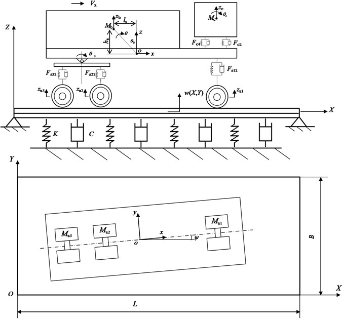
A three-directional (3D) coupled vehicle-road system is proposed in this work as shown in Fig. 1. A 23-DOF vehicle and a double-layer rectangular thin plate on viscoelastic foundation with four simply supported boundaries are employed to model vehicle and pavement. The upper layer of the plate models asphalt topping, the lower layer models base course, and the viscoelastic foundation stands for subgrade of the road. The material of topping and base course is assumed to be isotropy and elastic. The vehicle is able to moving on the road in different maneuver conditions, such as straight-line running at a constant speed, braking and turning. The origin of vehicle coordinate system (, , ) is located in the intersection between the roll axle and the vertical line passing vehicle center of gravity. is the vehicle’s yaw angle which describe the orientation of the vehicle. The static ground coordinate system (, , ) is also shown in Fig. 1, taking the stress neutral layer of pavement as coordinate axial , the lateral direction as coordinate axial and the vertical direction as coordinate axial .
Fig. 1The 3D coupled vehicle-road model
2.1. Equations of motion for the vehicle
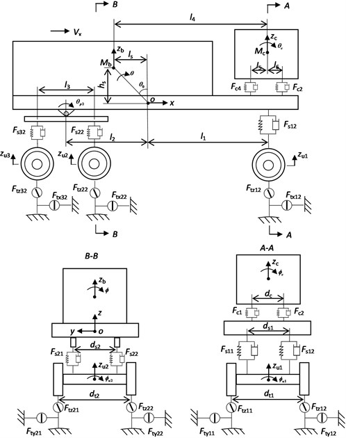
A nonlinear full-body model with 23-DOF for a three-axial heavy-duty truck is presented, as shown in Fig. 2. The vehicle is front wheel steered and rear wheel driven. , , represent the longitudinal and lateral displacements and the yaw angle of the full vehicle respectively. , , , , , stand for the vertical, pitch and roll displacements of driver cab and vehicle body. , (1,…, 3) denote the vertical and roll displacements of three wheel axles. , are the pitch angles of the left and right balancing pole on rear suspension. , , denote the masses of full vehicle, vehicle body and driver cab respectively. , are the vertical and longitudinal distance from the sprung mass center of gravity to the coordinate origin. , , are the front and rear wheel track width. , , are the lateral distance between left and right spring on front or rear suspension.
The movements of the heavy-duty vehicle are coupled with each other greatly. Eqs. (1)-(3) give the longitudinal, lateral and yaw dynamics of the full vehicle. Eqs. (4)-(6) give the vertical, roll and pitch dynamics of the sprung mass:
where , and are the steering angle of front wheel, the tire aligning torque, and the tire effective radius respectively. (1,…, 4) denotes the suspension forces between driver cab and vehicle body and can be expressed as:
For this heavy-duty vehicle, two hydraulic dampers are fixed on the left and right front suspension and the tandem balanced suspension doesn’t have any damper. The damper in vehicle suspension is one of the major factors influencing the vehicle handling and ride comfort and shows apparent nonlinearity, asymmetry and hysteresis. Many dynamic models for vehicle suspension damper have been proposed, including the parametric model [33], the equivalent parametric model [34, 35] and the fitted model [36, 37]. The fitted model is quite suitable to modeling the ascertained damper and the function of restoring force relate to velocity are fitted by the test data. In this work, the fitted model is used. The damping force of the damper on front axle can be described by a nonlinear segmented model:
where , , and are the relative velocity of cylinder and plunger, the damping coefficient, the asymmetry ratio and the exponent respectively. , , and are the damping force and relative velocity when the damper reaching saturation in tension or compression process. Eq. (8) is composed of three equations and modeled from the test data [38]. The first and third equations are dry friction damping models, which define the damping forces when the damper plunger arrives at the above or below limit position. The second equation describes the hysteresis viscous damping force when the plunger moves between the two limit positions. Here, 30893, 0.56, 0.16, 4119 N, 726 N, 0.12 m/s, 0.08 m/s. These parameters are obtained by fitting the measured data of the damper’s dynamic test. The test’s description and the related results were given by the author’s another work [38].
Fig. 2The full-body heavy vehicle model with 23-DOF
Using model Eq. (8) to calculate the damping force, the front suspension forces are expressed by:
where , are the left and right damping force of front suspension. The relative velocities of left and right damper are obtained by and .
In order to represent the frictional property of leaf spring, the damping forces of tandem balanced suspension are modeled linearly. The suspension forces between middle or rear axle and vehicle body are expressed by:
Eq. (11) gives the pitch motions of the balancing poles:
Here, the subscript 1, 2 stands for the left and right balancing pole of rear suspension.
The vertical, roll and pitch motions of the cab are formulated by:
The vertical and roll motions of three axles and the wheel rotating rates are given by:
where, and (1,…, 3, 1, 2) are the driving torque and braking torque of six wheels. The subscript stands for the front, middle or rear axle, and stands for the left or right wheel.
2.2. The three-directional tire forces
The square nonlinear tire model [39] is used to calculate the vertical tire forces:
where and are the linear tire vertical stiffness and damping coefficient respectively. is the square nonlinear stiffness coefficient. are the vertical tire displacements, which can be gained from the axle vertical and roll displacements:
are the road surface roughness and is the pavement displacement of the point under a wheel. The pavement displacements equations will be derived in Section 2.3 and given by Eq. (29). The positions of vehicle mass center and in the ground coordinate system are decided by vehicle velocities and yaw angle:
Then, the positions of wheels mass center and in the ground coordinate system can be calculated by:
where, (1,…, 3) are the longitudinal distances of three axles. .
The tire-road contact characteristic is one of the key issues to affect the vehicle dynamics and pavement dynamics. Many mathematical models of tire envelopment were proposed to model vertical tire force and tire-road contact characteristic during the past decades [40, 41]. These tire models can be divided into the point-contact model and the area-contact model.
The point-contact model can estimate vertical tire force with enough accuracy for long wavelength and small amplitude road surface irregularities and has been used widely [42, 43]. On large obstacles the point-contact model typically over predicts tire response, because it follows the contour of the road for rapid changes in elevation when a real tire would lose contact. The area-contact model offers a distinct improvement over the point contact model for discrete surface irregularities or short wavelength surface irregularities, but it uses too much computation time for practical application in responses calculations and also requires mechanical tire properties that are very specific to a given tire. For the asphalt concrete pavement in this work, it is assumed that there are no sharp discontinuities such as joints or potholes. To obtain trade-off between accuracy and efficiency requirements, the simple point-contact model is used here, as expressed by Eq. (15).
When the wheel jumps away the road surface, the vertical tire force obtained by Eq. (15) will become negative, while the tire force will become zero for the real tire. In order reflect the tire jump correctly, the vertical tire force is set to zero once the value obtained by Eq. (15) being negative.
Based on Gim tire model [44, 45], the lateral and longitudinal tire forces are described by:
where:
are the longitudinal and lateral wheel slip ratio. Here, are the slip angles of wheels, which is expressed by:
and is the turning angle of the front wheel. In addition:
are tire parameters related to slip ratios. , and are road adhesion coefficients. , and are the vehicle running speed, and the tire longitudinal and lateral stiffness respectively.
2.3. Equations of motion for the road
The road pavement height, elastic modulus, shear modulus, Poisson ratio and density are symbolized by , , , , , , , , and . The double-layer thin plate’s stresses for the linear elastic material are:
where , , are vertical-varied function of elastic modulus, shear modulus and Poisson ratio.
One may obtain the stresses of the double-layer plate satisfying the following functions:
where is curvature radius of stress neutral layer.
Since stress of neutral layer is zero, it can be gained:
Substituting Eq. (22) into Eq. (23), one gets:
where, is the distance between stress neutral layer and the upper surface of the double-layer plate.
The position of stress neutral layer can be obtained from Eq. (24):
Partial differential equation of the double-layer thin plate on viscoelastic foundation subjected by moving vehicle loads can be derived by elastic dynamics theory:
where:
and (1,…, 3, 1, 2) is the three-directional tire forces acting on road pavement, which may be expressed by:
where, and are longitudinal and lateral positions of tire respectively. , , , , are tire forces of six wheels, which may be expressed in road coordinate system by:
where, is the tire effective radius. are the orientation angles of wheels, which may be given by:
and , , are pneumatic trail, lateral offset and lateral deformation of tires, which need to be calculated in real time by:
here, is the tire lateral stiffness and is the tire footprint length.
Displacement of double-layer thin plate with four simply supported boundaries can be expressed as:
where, and are the pavement’s length and width.
Substituting Eq. (31) into Eq. (26) leads to residual value :
By limiting residual value the following equation can be get by Galerkin’s method:
By simplifying the above equation, Eq. (26) can be discretized as a set of ordinary differential equations:
where 1,…, , 1,…, and:
2.4. Three-dimensional interaction between the vehicle and road
According to Eq. (15), the vertical contact forces between tires and pavement are related not only to tires vertical motion and road surface roughness, but also to road vibrations at the contact points between tires and pavement. It is also noticed from Eqs. (16), (17) that the lateral and longitudinal tire forces are coupled with the vertical tire forces and vehicle responses. In addition, Eqs. (31) and (34) show that the pavement displacements are coupled with the three-dimensional tire forces and wheel positions. Consequently, the vehicle system equations Eqs. (1)-(6) and Eqs. (11)-(14) are coupled with the road system equations Eq. (34) through three-directional tire forces. Thus, these equations compose the first-order and second-order ordinary differential equations of the 3D-coupled vehicle-road system.
Some scholars think that the tire deformation is much bigger than the road vibration and it’s not need to research the vehicle-road interaction. However, the static deformation of the tire is caused by static tire loads and the dynamic deformation is caused by the road surface roughness and road vibration. Once the simulation begins, the static and dynamic deformation occur, the tire vibrates attenuately and arrives to the static balance position quickly. Then the tire will vibrate around the balance position. Thus vehicle-road interaction depends on the relation of road surface roughness and road vibration, and should not be neglected when the vehicle running on the smooth road. It’s also necessary to research the influence of 3D vehicle-road interaction on vehicle and road dynamics when the vehicle turning or braking.
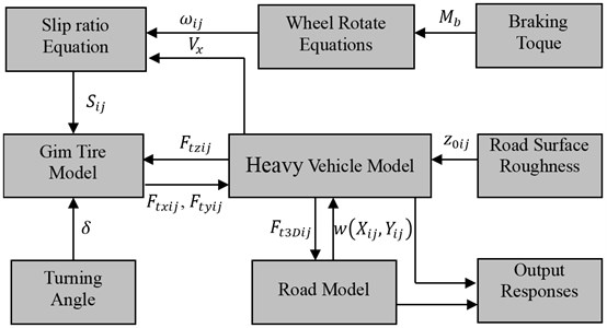
Due to the time variability, nonlinearity and high-dimensional property of this system, the closed-loop system equations are solved numerically by the quick integration method [46, 47] and the Runge-Kutta method of order four. The simulation process of this 3D vehicle-road system is shown in Fig. 3.
Fig. 3The simulation process of the 3D-coupled vehicle-road system
As a comparison, the vertical coupled and uncoupled vehicle-road model are also built. For the vertical coupled model, only the vertical tire forces act on the road and the right hand of Eq. (34) is expressed by:
For the uncoupled model, the vertical tire force doesn’t consider the effect of road vibration and is given by:
3. Comparison of responses of 3D coupled, vertical coupled and uncoupled vehicle-road models
In order to analyze the vehicle-road interaction using this proposed 3D coupled vehicle-road model, the computation method and the vehicle-pavement coupled model should be verified. However, it is very difficult to measure the vehicle and road dynamic responses simultaneously when a vehicle running on a road, especially when the vehicle turning, making a lane-change or braking. Due to lack of the test data of vehicle-road dynamics on every driving situation same to the simulation, only some simulation results were validated by experiments. Limited by the technical and economic conditions, we only obtained the test data of vehicle responses when the vehicle running at a constant speed along a straight line. By comparing with this test data, the validation of the 3D-coupled vehicle model has been given in the author’s another work [48]. In order to add confidence to the validity the road model, the road responses simulated by the vehicle-pavement coupled model was compared with the simulation results of Wu [21], using the same parameters and boundaries conditions to Wu’s model. The comparison results were given in the author’s previous work [30].
As many scholars think, simulation is also a useful and economic method to research vehicle and road dynamics when the driving situations are difficult or dangerous to achieve. Compared with the analytical method, the simulation method is also convenient and flexible to discuss the engineering problem modeled by high-dimensional equations. As follows, the property of 3D vehicle-road interaction will be simulated in different driving situations.
Parameters for the heavy vehicle system are chosen according to a heavy truck with full load which was used in the field test [48]:
1115 kg, 15797 kg, 20440 kg, 136×103 kg m2, 5.20 m, 1.15 m, 1.3 m, 4.83 m, 1.2 m, 1.0 m, 0.778 m, 0.52 m, 997.5 kN/m, 4000 N∙s/m, 2200 kN/m, 6300 N∙s/m, 373.8 kN/m, 454.6 kN/m (2, 3, 1, 2), 0.1, 1.9 m, 0.42 m, 0.01, 0.9, 0.15, 74.9 kN/m, 44.6 kN/m, 1985 N∙s/m, 1185 N∙s/m, 251.38 kN/m, 40 kN∙s/m, 1100 kN/m, 3500 N∙s/m, 186.9 kN/m, 227.3 kN/m.
Parameters for the pavement and foundation are chosen as follows [30, 31]:
0.1 m, 0.25, 1600 MPa, 2.5×10³ kg/m3, 0.2 m, 700 MPa, 0.25, 2.2×10³ kg/m3, 48×106 N/m3, 0.3×10⁶ N∙s/m2, 15 m/s, 95 m, 15 m. The random road roughness is B-class according to GB/T 7031-2005/ISO 8608:1995 [49] and is generated using the method of Liu [50].
Four driving maneuvers are simulated, including straight-line driving at a constant speed, straight-line braking, and curve driving at a constant speed and combined steering and braking. By comparing the responses of the road and vehicle obtained by 3D coupled, vertical coupled and uncoupled models, the effects of coupling action on responses are analyzed.
Fig. 4Pavement displacements when straight-line driving at Vx= 15 m/s
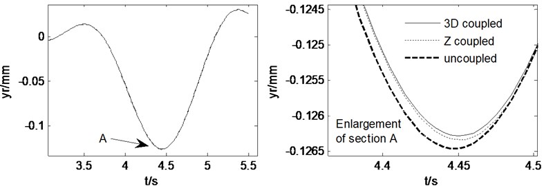
Fig. 5Vehicle responses when straight-line driving at Vx= 15 m/s
3.1. Straight-line driving at a constant speed
Letting the heavy vehicle runs along a straight-line at a constant speed of 15 m/s, the pavement displacements and vehicle responses induced by tire forces can be obtained from three models, 3D coupled, vertical coupled ( coupled) and uncoupled vehicle-road models, as shown in Fig. 4 and Fig. 5. It may be noticed from Fig. 4 that the difference between 3D coupled model and coupled model is slight and the pavement displacement decreases 0.2 % after considering the vehicle-road coupling action. In these three models, the 3D coupled model leads to the smallest pavement displacement. Fig. 5 shows that the effects of vehicle-road coupling on vehicle responses are great, but the difference between 3D coupled model and coupled model is still slight. After considering the vehicle-road coupling action, the peak value of longitudinal acceleration of vehicle body, vertical accelerations of vehicle body and cab increases 275 %, 204 % and 145 % respectively. Both 3D and vertical vehicle-road coupling also lead to obvious increase of vehicle lateral acceleration and yaw rate. However, in the case of straight-line driving, the lateral acceleration and yaw rate of the vehicle are too small to be considered.
Fig. 6Pavement displacements when straight-line braking with Mz= –56500 N∙m
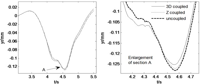
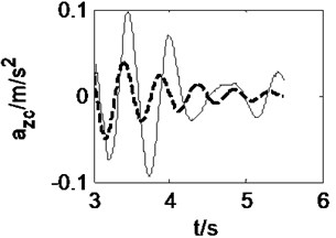
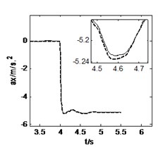
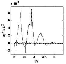
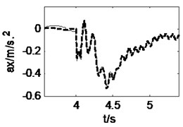
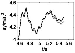
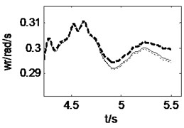
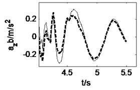
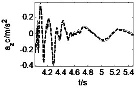
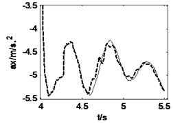
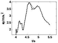
Fig. 7Vehicle responses when straight-line braking with Mz= –56500 N∙m
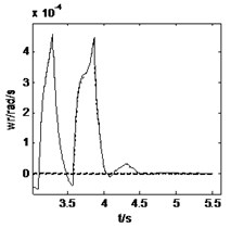
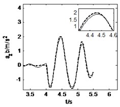
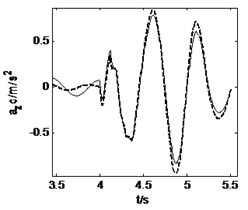
3.2. Straight-line braking
The vehicle moves along a straight-line at an initial speed of 15 m/s and is braked with a braking torque 56500 N∙m at the time of 4 s. The road and vehicle responses are calculated from three models, as shown in Fig. 6 and Fig. 7. It can be obtained from these two figures that the 3D and vertical coupling action leads to 2.1 % and 0.8 % decrease of the pavement displacement respectively. Hence, when the vehicle is braking, the influence of 3D vehicle-road coupling action on pavement displacement is enlarged. In addition, the vehicle response difference between 3D coupled model and coupled model is also very little. Compared with the uncoupled model, the two coupled vehicle-road models result in the peak value of longitudinal acceleration of vehicle body, and vertical accelerations of vehicle body and cab decreases 0.2 %, 5.0 % and 7.2 % respectively. It should be noted that the vehicle-road coupling causes a contrary impact on longitudinal vertical vehicle responses when vehicle is braking. However, the effects of vehicle-road coupling on the lateral acceleration and yaw rate are similar so long as the vehicle runs along a straight-line.
Fig. 8Pavement displacements when curving driving with δ= 0.15
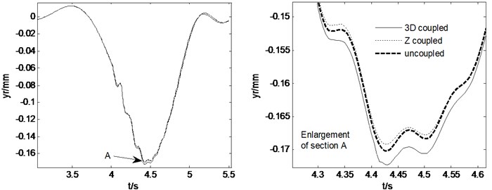
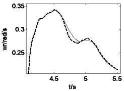
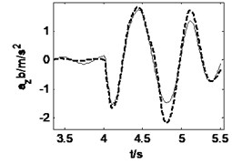
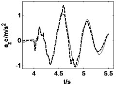
Fig. 9Vehicle responses when curve driving with δ= 0.15
3.3. Curve driving at a constant speed
When the vehicle is running along a straight-line at a constant speed of 15 m/s, a front wheel steering angle of 0.15 rad is input at 4 s, and then the curve driving begins. The pavement displacements and vehicle responses are calculated using 3D coupled, vertical coupled and uncoupled vehicle-road models respectively, as shown in Fig. 8 and Fig. 9. It can be seen from Fig. 8 that the 3D and vertical coupling action result in 1.2 % and –0.7 % variation of the pavement displacement. It is interesting that the effect of vertical vehicle-road coupling action on pavement displacement is the same as the case of straight-line driving, but the effect of 3D vehicle-road coupling action is contrary. It may be implied that the influence of lateral tire forces on pavement displacement is contrary to that of vertical and longitudinal tire forces. Fig. 9 shows that the vehicle response difference between 3D coupled model and coupled model is also tiny. With the coupling action considered, the peak value of longitudinal and vertical accelerations of vehicle body, the vertical accelerations, the lateral acceleration and yaw rate of cab changes –3.8 %, +31.2 %, +15.1 %, –0.9 %, +0.03 % respectively. Compared with the condition of straight-line driving at a constant speed, it is found that curve driving will enhance the influence of vehicle-road coupling on lateral vehicle responses.
Fig. 10Pavement displacements when combined steering and braking with δ= 0.15, Mz= –56500 N∙m
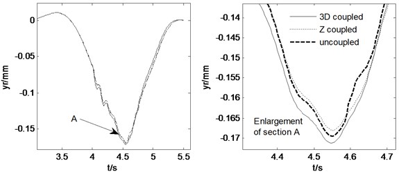
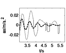
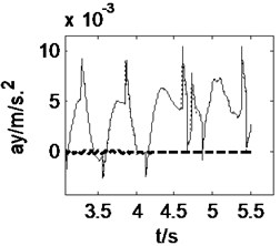
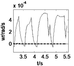
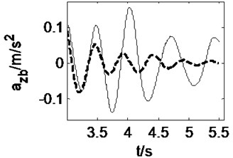
Fig. 11Vehicle responses when combined steering and braking with δ= 0.15, Mz= –56500 N∙m
3.4. Combined steering and braking
During the combined steering and braking driving maneuver, the heavy vehicle is input a front wheel steering angle 0.15 and a braking torque –56500 N∙m simultaneously when 4 s. The road roughness is B-class and the initial vehicle speed is 15 m/s. Fig. 10 and Fig. 11 show the road and vehicle responses obtained by the three vehicle-road models. It can be found from Fig. 10 that the 3D and vertical coupling action cause 1.1 % and –0.9 % change of the pavement displacement, and the pavement displacement obtained by 3D coupled model is the greatest. It should be noted again that the braking causes the decrease of the variation ratio. In addition, the vehicle response difference between 3D coupled model and coupled model is also tiny. With the coupling action considered, the peak value of longitudinal acceleration, vertical accelerations of vehicle body and cab, lateral acceleration and yaw rate increases 0.2 %, –20.6 %, –24.3 %, –0.6 %, –0.3 % respectively. Therefore, in the combined steering and braking driving maneuver, the effect of vehicle-road coupling arrives at obvious impacts on three-directional vehicle responses and can’t be neglected.
By comparing the results of above four driving conditions, it may be summarized that:
1) In different driving conditions, the vehicle response difference between 3D coupled model and coupled model is always tiny, but the difference between coupled and uncoupled model is too big to be neglected. Therefore, both 3D coupled model and vertical coupled model are good enough to predict vehicle responses accurately.
2) In straight-line driving condition, the pavement displacement obtained from 3D coupled model is smaller than that from vertical coupled and uncoupled model. But in curve driving condition, the pavement displacement predicted by 3D coupled model is bigger than those by the other two models. Whether in straight-line or curve driving condition, the vertical coupled model always obtains a smaller pavement displacement than the uncoupled model. Hence, the 3D coupled model is the most suitable for calculating road responses accurately.
4. Effects of system parameters on 3D vehicle-road interaction
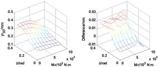
When a vehicle runs on a road, it may meet a lot of vehicle driving conditions and road type. Thus it is necessary to research the effects of road and vehicle parameters on vehicle-road interaction. Since the effects of vehicle and road parameters on vertical vehicle-road interaction have been given in detail by the authors’ previous works [30-32], this work only puts emphasis on the effects of parameters on 3D vehicle-road interaction. During simulation, six parameters are selected, including the front wheel steering angle, the braking torque, the nonlinear coefficient of vertical tire stiffness, the vehicle running speed, the road surface roughness and the road type. The pavement displacement peak value and the difference between the results of 3D coupled model and vertical coupled model are calculated with different values of parameters, as shown in Figs. 12-15.
Fig. 12 shows that the rise of steering angle will increase amplitude of the pavement displacement, but a big braking torque will reduce the amplitude of pavement displacement. With the increase of front wheel steering angle or braking torque, the result difference between 3D coupled model and vertical coupled model also increases. Thus, during the maneuver of sharp steering or emergency braking, the role of 3D vehicle-road interaction is enhanced.
Fig. 12Effects of front tire turning angle and braking torque
From Fig. 13, it can be seen that a high vehicle speed increases the amplitude of pavement displacement. At the vehicle speeds higher than 60 km/h, the effect of the nonlinear tire coefficient increases substantially. In addition, with the increase of the vehicle speed or the nonlinear tire coefficient, the difference between 3D coupled model and vertical coupled model increases but is accompanied by occasional fluctuation. At the vehicle speeds higher than 60 km/h, the effect of the nonlinear tire coefficient increases substantially. Thus the nonlinear tire stiffness should not be neglected at higher vehicle speeds.
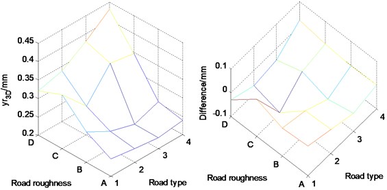
In Fig. 14, the road roughness goes up from A to D class [39], and road type 1 to 4 stand for dry asphalt road, wet asphalt road, snow surface road and ice surface road respectively. The surface adhesion coefficients of these four road types are 0.95, 0.5, 0.15 and 0.07. From Fig. 14, it can be seen that a rough road will lead to a bigger pavement displacement, and the pavement displacement is the biggest on rough ice surface road. However, on smooth dry asphalt road the difference between the results of 3D coupled model and vertical coupled model is the biggest. The reason might be that a big road surface adhesion coefficient leads to the large longitudinal and lateral tire forces, which will reinforce the effect of 3D vehicle-road coupling. Moreover, in the smooth road with small surface roughness, the ratio of pavement vibration to road excitation is bigger than that in rough road and thus the effect of vertical vehicle-road coupling is enhanced.
Fig. 13Effects of square nonlinear coefficient of tire stiffness and vehicle running speed
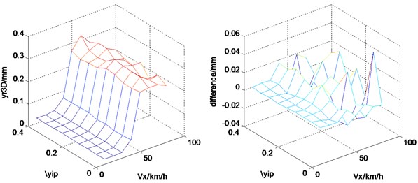
Fig. 14Effects of road roughness and road type
5. Conclusions
An innovative three-directional coupled vehicle-road model is built for studying the properties of three-directional (3D) interaction between vehicle and road. It has been found that:
1) Both the 3D coupled model and the vertical coupled model are good enough to predict vehicle responses accurately, but the 3D coupled model is the most suitable for calculating road responses accurately.
2) During the maneuver of sharp steering or emergency braking, the road response difference between 3D coupled model and coupled model is enhanced and the 3D vehicle-road interaction should be considered.
3) When a vehicle runs on a road with small surface roughness and big adhesion coefficient, the difference between results of 3D coupled model and vertical coupled model is obvious and the 3D vehicle-road interaction should be considered.
4) With the increase of the vehicle speed or the nonlinear tire coefficient, the difference between 3D coupled model and vertical coupled model increases but is accompanied by occasional fluctuation. The nonlinear tire stiffness should not be neglected at higher vehicle speeds.
In this work, the value of tire stiffness is selected as to the normal air pressure in the tire and the square nonlinear tire model is applied. In fact, a finite element tire model can consider the effect of air pressure in the tire and the tire structure better. However, how to connect a finite element tire model with a vehicle model and a road model is still a challenging problem, which is also our future research direction. In addition, the vehicle-road tests on complicated driving situations including lane change, turning and braking need to be fulfilled so as to validate the simulation results.
References
-
Sha Q. L. Highway Asphalt Pavement Premature Damage and Prevention. China Communications Press, Beijing, 2001.
-
Gillespie T. D. Effects of Heavy-Vehicle Characteristics on Pavement Response and Performance. Transportation Research Board, Report Number UMTRI-92-2, 1993, p. 1-126.
-
Cebon D. Interaction between Heavy Vehicles and Roads. SAE 930001, SEA/SP-93/951, 1993.
-
Cole D. J. Truck suspension design to minimize road damage. Proceedings of the Institution of Mechanical Engineers. Part D: Journal of Automobile Engineering, Vol. 210, 1996, p. 95-107.
-
Markow M. J., Brademeyer B. D. Analyzing the interactions between dynamic vehicle loads and highway pavements. Transportation Research Record, Vol. 1196, 1996, p. 161-169.
-
Myers L. Measurement of contact stress for different truck tire types to evaluate their influence on near surface cracking and rutting. Transportation Research Record Vol. 1655, 1999, p. 175-184.
-
Sun L., Cai X. M., Yang J. Genetic algorithm-based optimum vehicle suspension design using minimum dynamic pavement load as a design criterion. Journal of Sound and Vibration, Vol. 301, Issues 1-2, 2007, p. 18-27.
-
Lu Y. J., Yang S. P., Li S. H. Numerical and experimental investigation on stochastic dynamic load of a heavy duty vehicle. Applied Mathematic Modeling, Vol. 34, Issue 10, 2010, p. 2698-2710.
-
Chen Y. K., He J., King M. Comparison of two suspension control strategies for multi-axle heavy truck. Journal of Central South University, Vol. 20, Issue 2, 2013, p. 550-562.
-
Jorge B. S., Joseph C., Carl L. M. Summary Report on Permanent Deformation in Asphalt Concrete. Transportation Research Board Business Office, Washington, 1991.
-
Transportation Research Broad. Strategic Highway Research Program 2 [EB/OL]. http://www.trb.org/SHRP2, 2009.
-
Hardy M. S. A., Cebon D. Response of continuous pavements to moving dynamic loads. Journal of Engineering Mechanics, Vol. 119, Issue 9, 1993, p. 1762-178.
-
Deng X. J., Sun L. Study on the Dynamics of a Vehicle-Ground Pavement Structure System. China Communications Press, Beijing, 2000.
-
Kim S. M., McCullough B. F. Dynamic response of a plate on a viscous Winkler foundation to moving loads of varying amplitude. Engineering Structure, Vol. 25, 2003, p. 1179-1188.
-
Jeongho O., Fernando E. G., Lytton R. L. Evaluation of damage potential for pavements due to overweight truck traffic. Journal of transportation Engineering, Vol. 133, Issue 5, 2007, p. 308-317.
-
Hryniewicz Z., Kozioł P. Wavelet-based solution for vibrations of a beam on a nonlinear viscoelastic foundation due to moving load. Journal of Theoretical and Applied Mechanics, Vol. 51, Issue 1, 2013, p. 215-224.
-
Ding H., Shi K. L., Chen L. Q., et al. Dynamic response of an infinite Timoshenko beam on a nonlinear viscoelastic foundation to a moving load. Nonlinear Dynamics, Vol. 73, Issues 1-2, 2013, p. 285-298.
-
Fang X. Q., Yang S. P., Liu J. X. Dynamic response of road pavement resting on a layered poroelastic half-space to a moving traffic load. International Journal for Numerical and Analytical Methods in Geomechanics, Vol. 38, Issue 2, 2014, p. 189-201.
-
Markow M. J., Hedrick J. K., Brademeyer B. D. Analyzing the interactions between dynamic vehicle loads and highway pavement. Transportation Research Record, Vol. 1196, 1988, p. 161-169.
-
Collop A. C., Cebon D. Parametric study of factors affecting flexible-pavement performance. Journal of Transportation Engineering, Vol. 121, Issue 6, 1995, p. 485-494.
-
Wu C. P., Shen P. A. Dynamic analysis of concrete pavements subjected to moving loads. Journal of Transportation Engineering, Vol. 122, Issue 5, 1995, p. 367-373.
-
Mamlouk M. S. General outlook of pavement and vehicle dynamics. Journal of Transportation Engineering, Vol. 123, Issue 6, 1997, p. 515-517.
-
Siddharthan R. V., Peter J. Y., Sebaaly E. Pavement strain from moving dynamic 3D load distribution. Journal of Transportation Engineering, Vol. 124, Issue 6, 1998, p. 557-566.
-
Liu C., McCullough B. F., Oey H. S. Response of a rigid pavement to vehicle-road interaction. Journal of Transportation Engineering, Vol. 126, Issue 3, 2000, p. 237-242.
-
Metrikine A. V., Verichev S. N., Blaauwendraad J. Stability of a two-mass oscillator moving on a beam supported by a viscoelastic half-space. International Journal of Solids and Structures, Vol. 42, 2005, p. 1187-1207.
-
Giuseppe M., Alessandro P. Response of beams resting on a viscoelastically damped foundation to moving oscillators. International Journal of Solids and Structures, Vol. 44, 2007, p. 1317-1336.
-
Shi X. M., Cai C. S. Simulation of dynamic effects of vehicles on pavement using a 3D interaction model. Journal of Transportation Engineering, Vol. 135, Issue 10, 2009, p. 736-744.
-
Taheri A., Obrien E. J., Collop A. C. Pavement damage model incorporating vehicle dynamics and a 3D pavement surface. International Journal of Pavement Engineering, Vol. 13, Issue 4, 2012, p. 374-383.
-
Ding H., Yang Y., Chen L. Q. Vibration of vehicle–pavement coupled system based on a Timoshenko beam on a nonlinear foundation. Journal of Sound and Vibration, Vol. 333, Issue 24, 2014, p. 6623-6636.
-
Yang S. P., Li S. H., Lu Y. J. Investigation on the dynamic interaction between a heavy vehicle and road pavement. Vehicle System Dynamics, Vol. 48, Issue 8, 2010, p. 923-944.
-
Li S.H., Yang S.P., Chen L.Q. Effects of parameters on dynamic responses for a heavy vehicle-pavement-foundation coupled system. International Journal of Heavy Vehicle Systems, Vol. 19, Issue 2, 2012, p. 207-224.
-
Yang S. P., Chen L. Q., Li S. H. Dynamics of Vehicle-Road Coupled System. Science Press, Beijing and Springer-Verlag, Berlin Heidelberg, 2015.
-
Titurus B., Bois J. D., Lieven N. A method for the identification of hydraulic damper characteristics from steady velocity inputs. Mechanical Systems and Signal Processing, Vol. 24, 2010, p. 2868-2887.
-
Besinger F. H., Cebon D., Cole D. J. Damper models for heavy vehicle ride dynamics. Vehicle System Dynamics, Vol. 24, Issue 1, 1995, p. 35-64.
-
Zubieta M., Elejabarrieta M. J., Bou-Ali M. M. Characterization and modeling of the static and dynamic friction in a damper. Mechanism and Machine Theory, Vol. 44, 2009, p. 1560-1569.
-
Worden K., Hickey D., Haroon M. Nonlinear system identification of automotive dampers: a time and frequency-domain analysis. Mechanical Systems and Signal Processing, Vol. 23, 2009, p. 104-126.
-
Li S. H., Lu Y. J., Li L. Y. Dynamical test and modeling for hydraulic shock absorber on heavy vehicle under harmonic and random loadings. Research Journal of Applied Sciences, Engineering and Technology, Vol. 4, Issue 13, 2012, p. 1903-1910.
-
Li S. H., Ren J. Y. Driver steering control and full vehicle dynamics study based on a nonlinear three-directional coupled heavy-duty vehicle model. Mathematical Problems in Engineering, 2014, p. 352374.
-
Ji X. W., Gao Y. M. The dynamic stiffness and damping characteristics of the tire. Automotive Engineering, Vol. 5, 1994, p. 315-321.
-
Captain K. M., et. al. Analytical Tire models for dynamic vehicle simulation. Vehicle System Dynamics, Vol. 8, 1979, p. 1-12.
-
Zegelaar P. W. A. The Dynamic Response of Tyres to Brake Torque Variations and Road Unevenness. Ph.D. Dissertation, Delft University of Technology, 1998.
-
Rutka Arunas, Sapragonas Jonas The role of a tire in vehicle and road interaction. Transport, Vol. 17, Issue 2, 2002, p. 39-45.
-
Miege Arnaud Tyre Model for Truck Ride Simulations. University of Cambridge, 2002.
-
Gim G., Nikravesh P. E. A three dimensional tire model for steady-state simulations of vehicles. SAE, Vol. 102, Issue 2, 1993, p. 150-159.
-
Zhuang J. D. Principles of Automobile Tire. Beijing Institute of Technology Press, Beijing, 1996.
-
Zhai W. M. Vehicle-Track Coupled Dynamics. China Railway Publishing House, Beijing, 2002.
-
Zhai W. M. Two simple fast integration methods for large-scale dynamic problems in engineering. International Journal for Numerical Methods in Engineering, Vol. 39, 1996, p. 4199-4214.
-
Li S. H., Yang S. P., Chen L. Q. Modeling and dynamic analysis of a nonlinear heavy vehicle with three-directional coupled motions. Journal of Vibration and Shock, Vol. 33, Issue 22, 2014, p. 131-138.
-
GB/T 7031-2005/ISO 8608:1995. Mechanical Vibration-Road Surface Profiles – Reporting of Measured Data. 2005.
-
Liu X. D., Deng Z. D., Gao F. Research on the method of simulating road roughness numerically. Journal of Beijing University of Aeronautics and Astronautics, Vol. 29, Issue 9, 2003, p. 843-846.
About this article

The National Natural Science Foundation of China (11472180) and the New Century Talent Foundation of Ministry of Education (NCET-13-0913) support this work.
