Abstract
An integrated control algorithm of the differential braking and the active suspension to improve yaw and rollover stability of vehicles with mechanical elastic wheel (ME-Wheel) is developed. By simplifying the structure of ME-Wheel, a fitting tire model named brush model is constructed. Then, a nonlinear 8-DOF vehicle model with ME-Wheel is built up for rollover prevention, which utilizes a predictive load transfer ratio (PLTR) as the rollover index and a Kalman filter is used to eliminate the measurement noise. In order to design an integrated control algorithm, fuzzy proportional-integral-derivative (PID) methodology is adopted by simultaneous control of the yaw and roll motions. The proposed algorithm, based on the idea that makes yaw stability controller and roll stability controller work independently first, then unifies by way of weight according to fuzz control, after that, brake force distributor selects single efficient braking wheel to achieve yaw moment and one of the front braking wheels with varying brake pressure to achieve the desired brake torque and the wheel slip regulator is designed with sliding mode control technique to prevent the wheels from locking; and the active suspension system alters the stiffness of the active suspension to prevent rollover. Simulation results show that the integrated yaw and rollover stability control system could improve the handing stability of vehicle under the limit driving conditions, and prevent rollover happening.
Highlights
- The 8-DOF nonlinear vehicle model is built up and the results show that the model is effective compared with the Carsim outputs and test results.
- Based on brush modeling theory, longitudinal and steady-state cornering mixed model of ME-Wheel are established and tested.
- The rollover index of PLTR can provide a time-advanced measurement of rollover prediction and its accuracy is verified by virtual tests.
- The integrated YSC+RSC controller based on Fuzzy-PID with rollover evaluation index of PLTR shows good control performance and improve the rollover and yaw stability of the vehicle.
1. Introduction
It is well known that automobile side slip and rollover are basically typical traffic safety problems. Vehicle driving safety is mainly dependent on yaw and rollover stability. In the last decade, vehicle electronic stability control (ESC) has attracted wide interest in research and been widely applied on vehicle, especially on passenger car [1-6]. However, most of the ESC systems presently adopt active yaw moment control to achieve vehicle yaw stability and they work well only with the tire forces within the friction limit. Direct yaw moment control (DYC) is one of the typical methods for yaw stability control where extensive researches have been conducted with different algorithms and strategies as reported in [7, 8]. DYC can be implemented by active braking, which the required yaw moment is generated by the designed controller and controls the desired yaw rate.
For off-road vehicle with high center of gravity (CG), rollovers might still occur easily even with ESC to deal with vehicle lateral stability [9]. Thus, many approaches have been adopted for rollover prevention, such as active differential braking [9, 10], active suspension [11-13] and together with active suspension and differential braking [14]. By braking the target wheels, active braking system can decrease the velocity of a vehicle and lateral acceleration when the vehicle is in danger of rollover. A switched suspension setting was shown in [11] which used switched stable control and two settings of suspension to prevent rollover. Kamal [12] introduced a conceptual strategy that uses different actuating forces between the front and rear axle which causes a pitch motion along with the body roll to enhance handling of a vehicle during cornering maneuver while improving rollover stability. Facts proved that it’s more effective to prevent rollover by braking target wheels and altering active suspensions, simultaneously. Yim [14] designed a rollover prevention controller by active suspension and differential braking, which is robust to the variation of parameters.
To rollover stability control, it’s necessary to design a warning system. Rollover warning system predicts whether the vehicle has a risk of rollover in a period of time based on the current driving state of the vehicle. Rollover prediction systems have been studied by many researchers with several different means, such as the load transfer ratio (LTR) [15], the improved predictive lateral load transfer ratio (IPLTR) [16], the time-to-rollover (TTR) [17] and the matched time to rollover (MTTR) [18].
Meanwhile, for the design of vehicle yaw stability control (YSC) and rollover stability control (RSC), most methods were considered a certain situation and more attention was focused on the vehicle yaw stability when there is no danger of rollover. However, both vehicle yaw stability and rollover prevention control should be integrated in practice especially in critical steering maneuver course [19].
We should improve the function of ESC and make rollover stability as it’s another important control objective. To coordinate YSC and RSC effectively and realize both yaw and rollover stability to the utmost, it needs to realize integrated control of YSC and RSC [20]. The relationship between rollover prevention control and yaw stability control is complex and both are related to the complicated lateral dynamics of a vehicle. What’s more, road friction coefficient has an important significance on electronic control system [21]. It also should make the integrated control system adapt to any road conditions [22].
In order to overcome those limitations, this paper suggests an integrated control strategy by coordinate YSC and RSC and realize both yaw and rollover stability to the utmost. The integrated controller includes differential braking controller and active suspension controller.
Taking an off-road vehicle as the research object, whose parameters were given in Table 5. The rest of the paper is organized as follows: In Section 2, the vehicle model of 8-DOF is built up. Then the proposed control structure is presented in Section 3, followed by simulation results in Section 4. The summary of the work is given in Section 5.
2. Vehicle model
The vehicle studied in this paper is an off-road vehicle with ME-Wheel. This section describes an eight-degree-of-freedom nonlinear vehicle model, which includes the longitudinal motion, lateral motion, yaw motion, roll motion and 4 wheels’ rotations.
2.1. 8-DOF nonlinear vehicle model
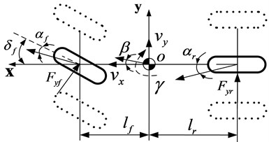
An 8-DOF nonlinear vehicle model is introduced considering the nonlinear tire force feature. The equations of body motion are illustrated in Fig. 1. The -axis is directed towards the longitudinal axis of body of the vehicle and the -axis is orthogonal to the -axis and passes through the centre of gravity (CG) and the vertical -axis passes through CG too.
The longitudinal motion is defined by the Eq. (1) as a balance function of -axis forces:
where is the vehicle total mass, is the vehicle sprung mass, is roll angle about -axle, is yaw rate about -axle, is the height of CG from roll center, is the longitudinal force of the th wheel in the vehicle coordinates ( 1, 2, 3, 4), , are the velocity at the CG along , .
The lateral motion is defined by the Eq. (2) as a balance function of -axis forces:
where and are the distance from CG to front and rear axle, respectively, and are the front and rear unsprung mass, respectively, is the lateral force of the th wheel.
Fig. 18-DOF nonlinear vehicle model
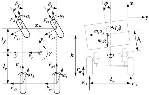
The yaw motion is defined by the Eq. (3) as a balance function of -axis force moments:
where is the yaw moment of inertia about -axis, is the wheel track width.
The roll motion is defined by the Eq. (4) as a balance function of x-axis force moments:
where and are the front and rear suspension roll stiffness, respectively, and are the front and rear suspension roll damping coefficient, respectively.
For the th wheel ( 1, 2, 3, 4), and, in the vehicle coordinates have the relationships with the tire forces , as follows:
for front wheel steering vehicle, we know, , 0, then:
For wheel th, the rotational dynamics can be formulated as:
where are angular velocities of 4 wheels, is the wheel moment of inertia, is the brake torque on each wheel.
2.2. Tire model
For the influence of simulation precision, tire force is an important factors. The non-linearity of the automobile model refers to the nonlinear tire characteristics. Fig. 2 shows the main components of the ME-Wheel.
Magic Formula proposed by Pacejka has been widely used in tire modeling. Compared with pneumatic tires, the longitudinal and lateral force calculations need some specific parameters and the characteristic data for non-pneumatic elastic wheel are incomplete because longitudinal and lateral slip of non-pneumatic elastic wheels need to be redefined by considering the longitudinal, lateral, and vertical deformations of treads and elastic supports [23]. Based on the above reasons, a relatively simple physical model, namely the brush model (Fig. 3), was selected to calculate the longitudinal and lateral force. The wheel deformation in contact with ground is shown in Fig. 4.
Fig. 2Structure of the ME-Wheel
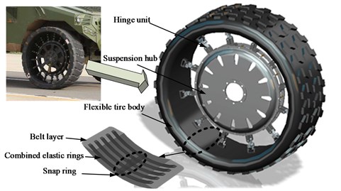
Fig. 3Simplified graphic of brush model
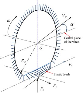
Fig. 4A schematic of the deformation of the elements of the tread in longitudinal direction
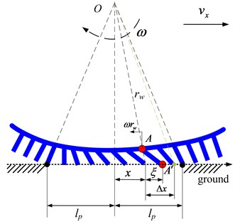
The longitudinal length of contact area is 2. As the role of longitudinal force in longitudinal direction of units , the bristle deformation is:
where is longitudinal displacement at pure rolling without any slip.
Define and practical longitudinal slip , then, . Longitudinal per unit force along the contact area can be expressed as:
Then, the longitudinal force can be expressed as:
where is the longitudinal stiffness of the elements of the tread. However, Eq. (10) never considers the conditions when longitudinal force is out of the limit of adhesion. The sketch of the strains along the tire contact area is shown in Fig. 5.
Fig. 5A sketch of the strains along the contact area of the tire
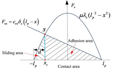
The front part of the whole contact area is adhesion area. is the critical point which breaks the contact area into two parts, sliding area and adhesion area. is the longitudinal coordinate. is the length of the sliding area. From the Fig. 5, longitudinal force can be expressed as:
Based on brush modeling theory, the longitudinal force along the whole contact area can be expressed as [23]:
The wheel deformation in contact with ground in lateral direction is shown in Fig. 6. is the critical point between the sliding area and the adhesion area, is the longitudinal coordinate of the point in contact area.
As the role of lateral force in lateral direction of brush units , bristle deformation is . Lateral per unit force along the contact area can be expressed as:
then:
where is the lateral stiffness of the tread elements. Then, lateral force can be expressed as:
Finally, the lateral force along the whole contact area can be expressed as [23]:
The experiments of dynamic mechanical characteristics of the ME-Wheel were conducted using a flatbed low-speed tire test rig as presented in Fig. 7.
Fig. 6A schematic of the deformation of the elements of the tread in lateral direction
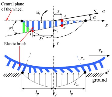
Fig. 7Experimental set-up for tire mechanical characteristics tests
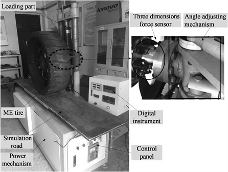
The specific steps of the tire mechanical properties test rig are as follows: First, demarcates the test bench and sets the angle of the test wheel to zero before experiment. Second, adjusts the test wheel to the specified slip angle by the angle adjustment mechanism and applies the desired load to the wheel by the loading part. Next, drives the simulated pavement moving from the test bench side to the other side at a stable translation speed by the power mechanism. Furthermore, sets sampling point and proper sampling range on simulated pavement and records the tire force of the wheel at each sampling point after the test wheel entering the sampling range by the data acquisition system. In the end, adjusts the vertical load or slip angle and repeats to test.
By analyzing the experimental data, a fitting model of half long grounding mark and lateral distribution stiffness along with vertical tire forces are established, respectively, as:
The parameters - and - are illustrated in Table 1, which were calibrated through tire force tests and the simulated results.
Table 1Fitted coefficient of brush model
–0.04 | 3.39 | 49.89 | –0.016 | 0.49 | 3.59 |
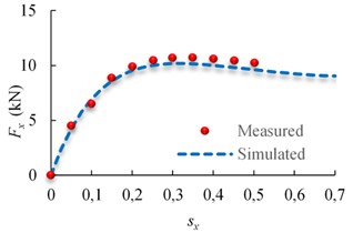
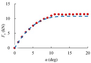
Multiple different longitudinal slip from 0 to 0.7 and different slip angle from 0 to 20 deg are applied to the ME-Wheel. The applied vertical load is 15 KN. The variation of longitudinal tire force with respect to the longitudinal slip and lateral tire force with respect to the slip angle are illustrated in Fig. 8.
Fig. 8Longitudinal and lateral tire force response
a)
b)
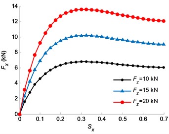
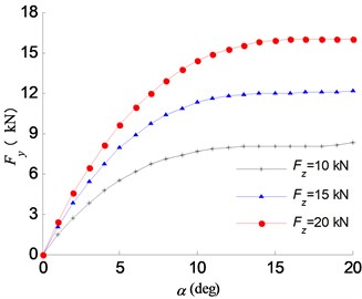
As for the cornering conditions, different rotational speeds and translational speeds are applied on the ME-Wheel and the applied vertical load is 10 kN, 15 kN and 20 kN, respectively. The variation of longitudinal tire force with respect to the longitudinal slip and lateral tire force with respect to the slip angle are illustrated in Fig. 9.
Fig. 9Tire force response at different vertical tire forces: a) Fx, b) Fy
a)
b)
The slip angles can be calculated by:
The normal tire force has significant effects on the vehicle handling and stability performance. The tire normal force calculation includes the load transfers due to the accelerations of longitudinal and lateral:
where are vertical tire forces of 4 wheels.
The longitudinal and lateral tire forces obtained by brush tire model need to be modified with the wheel slip angle and wheel slip ratio as follows:
3. Integrated control algorithm
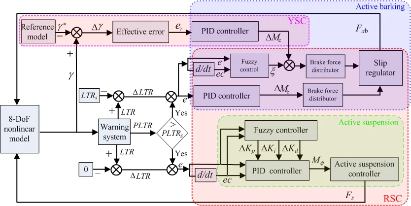
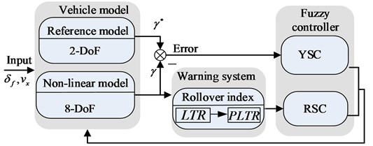
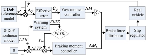
The assumed system structure, shown in Fig. 10, contains three vehicle modules, a rollover warning system and an integrated fuzzy controller of yaw moment and roll moment.
The shortcomings of rollover controller with active suspension are slow response of speed, poor real-time performance, and using differential braking control technology will make it up. In order to reduce the impact of the yawing stability by differential braking to the vehicle, a suspension controller is combined to adjust the posture of vehicle body, which can reduce the height of mass center and the size of the roll angle, and make the differential braking control system control the values of rollover index within the allowed range in a relatively short period of time.
Fig. 10Block diagram of the whole integrated control system
3.1. Rollover warning system
Rollover warning system predict whether the vehicle has a rollover risk in a period of time and LTR is one of the commonly used rollover index, which is formulated as [15]:
LTR represents load transfer within an axle and ranges between –1 to 1. If the vertical load of right wheels is equal to zero ( 0), the right wheels will lift off and –1.
By analyzing the roll stability mechanism of the vehicle, the LTR can be rewritten as [16]:
The PLTR is defined as follows:
where is the current time, is the preview time.
When the roll angle is very small, it can be assumed that , Substituting Eq. (23) into Eq. (24), then:
By 2-DOF bicycle model, the lateral acceleration can be further estimated as follows:
where:
The derivative of Eq. (26) can be written as:
where:
Then, the lateral acceleration derivative in the second term can be further rewritten as:
where is the steering angle, is the steering ratio ( 20).
Hence, substituting Eq. (28) into Eq. (25), the final form of PLTR is shown as follows:
If vehicle state parameters can be measured or estimated, it is easy to calculate the value of PLTR.
3.2. Fuzzy PID controller for active suspension system
It’s uncomfortable for people to have stiffer suspension for common driving conditions. However soft roll stiffness implies roll propensity. The active suspension system uses the signals from the vehicle and sends the altering of stiffness to the suspension. Stiffness of the suspension will make difference when the value of rollover index over the set value in order to reduce rollover propensity. Fig. 11 shows the block diagram of the active suspension control scheme.
Fig. 11Block diagram of the active suspension control scheme
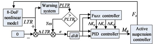
Identifying a good PLTR threshold is difficult because of dynamic changes and the off-road vehicle with high-CG. To achieve an enough time for rollover prevention system to prevent the vehicle from rollover, the threshold value of PLTRs is finally set as 0.7.
Fuzzy self-adjusting PID controller is the combination of PID controller with adjustable parameters (, , ) and fuzzy controller. Here, interval change of PID parameters is calculated utilizing fuzzy logic. The design of the active suspension controller is as follows:
The effective error e can be calculated as:
where:
When PLTR is smaller enough than , the controller doesn’t work. However, as roll angle gets bigger, PLTR is larger than , then, the control system start using the fuzzy PID controller. The fuzzy PID controller takes as error () and relative velocity as rate of change of error () and outputs adjustable PID parameters according to the requirement using fuzzy rules.
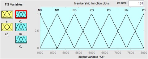
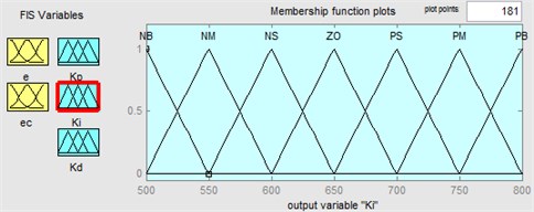
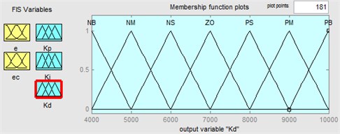
The four steps of a fuzzy logical controller are fuzzification, rule base design, approximate reasoning and defuzzification. First, fuzzification sets as PB (too high), PM (very high), PS (high), ZO (normal), NS (low), NM (very low), NB (too low). Gaussian membership functions are used for each variable. The two inputs of the fuzzy logic controller are: and . The membership functions are presented in Fig. 12. Fuzzy set “ZO” represents the rollover risk is in normal conditions, “PB” represents the rollover risk is in “high” conditions. Second, the fuzzy rules bases are composed of a set of if-then rules, which describe the relationships between state variables and control parameters. The fuzzy control rules can be referred to from the author’s previous work (Li et al., 2017). Third, after obtaining a final fuzzy set, it is required to defuzzify set to get a numerical output as the control signal. The most common defuzzifier is the center of area. In this work, mamdani type of inference method and centroid defuzzification method are used to design the fuzzy PID controller.
Fig. 12Membership functions in fuzzy logic controller for output variable: a) ∆Kp, b) ∆Ki, c) ∆Kd
a)
b)
c)
3.3. Integrated active braking control system
The integrated control algorithm of yaw and rollover stability based on active braking is developed. and PLTR can well reflect vehicle’s yaw and roll properties, which are selected as the followed variables. Fig. 13 shows the block diagram of the active braking control scheme.
Fig. 13Block diagram of the integrated active braking control scheme
The integrated braking control algorithms, based on the idea that independently decision make firstly and integrated by weight. In other words, making yaw stability controller (YSC) and roll stability controller (RSC) decide the needed yaw moment and brake torque independently first, then unifies the yaw moment and brake torque by way of weight.
For the design of YSC, a 2-DOF model is implemented to obtain the reference yaw rate. The yaw moment control is adopted to generate a desired yaw moment in order to reduce the yaw rate error between the reference and actual yaw rate.
Fig. 142-DOF vehicle dynamics model
The desired yaw rate response can be obtained by using the following equation [3]:
where:
The desired yaw rate (Eq. (33)) cannot be obtained if the road friction coefficient is not high enough. Thus, the desired yaw rate is:
The desired response of yaw rate can be rewritten as:
The corrective yaw moment and braking moment can be calculated by Eqs. (36)-(38) as:
For the accurate braking torque calculation, control parameters (, , ) are calculated utilizing model simulations. The effective error can be calculated as:
where , . Then, the additional moment can be formulated as:
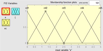
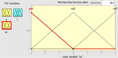
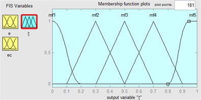
where is the weight coefficient of the yaw moment. There is another problem, how to get . When the PLTR is small enough, differential braking control system using yaw moment controller can satisfy the request. Therefore, the weighting is mostly on yaw moment controller. However, as roll angle gets bigger, PLTR is bigger than PLTRs, the control system still using yaw moment controller starts to become inaccurate. Hence, in this case, it is more efficient design a fuzzy controller. Such shift thus normally causes the braking system to be less sensitive for all sorts of driving scenarios. In this work, for the input errors of (), five conditions are considered for fuzzification which linguistic variables are assigned to these fuzzy and set as mf1 (too low), mf2 (low), mf3 (normal), mf4 (high), mf5 (too high). And for the input of , three conditions are considered for fuzzification and set as mf1 (low), mf2 (normal), mf3 (high). For the output, there were five levels for the altering: mf1 (too low), mf2 (low), mf3 (normal), mf4 (high), mf5 (too high). The membership functions are presented in Fig. 15. The fuzzy control rules are made in the form of Table 2.
Table 2Fuzzy control rules for ξ
mf1 | mf2 | mf3 | mf4 | mf5 | ||
mf1 | mf5 | mf4 | mf3 | mf2 | mf1 | |
mf2 | mf5 | mf4 | mf3 | mf2 | mf1 | |
mf3 | mf4 | mf3 | mf2 | mf1 | mf1 | |
Fig. 15Membership functions in fuzzy logic controller: a) e, b) ec, c) ξ
a)
b)
c)
3.4. The brake force distribute system
Brake force distributor aims to generate the yaw moment calculated from the yaw moment controller and braking moment calculated from roll stability controller.
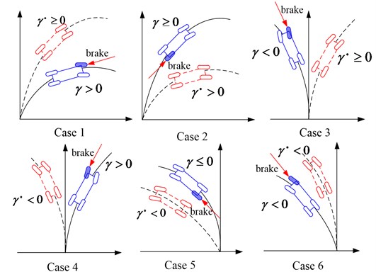
Yaw moment controller by distributing the brake force to the right wheel which is efficient is decided in Table 3 and roll moment controller by distributing the brake force to the target wheel which is efficient is decided in Table 4, correspondingly. The direct understanding of the yaw rare response comparisons with brake wheels decision is given in Fig. 16.
‘FL’, ‘FR’, ‘RL’ and ‘RR’ denote the front left wheel, front right wheel, rear left wheel and rear right wheel respectively.
The whole needed brake force is calculated by an integrated controller (yaw stability controller and roll stability controller) with a fuzzy controller.
Give the corrective yaw moment and a braking torque to stabilize the vehicle, if the target braking wheels are the same, and assuming that the brake force generated by the primary brake wheel on the front axle, this brake force can be calculated as:
Table 3Differential braking control decision for yaw stability
Case1 | 0 | 0 | FL | |
Case2 | 0 | 0 | RR | |
Case3 | 0 | 0 | FR | |
Case4 | 0 | 0 | FL | |
Case5 | 0 | 0 | RL | |
Case6 | 0 | 0 | FR |
Table 4Differential braking control decision for roll stability
Case1 | 0 | FL | |
Case2 | 0 | FR |
Fig. 16Yaw rare response comparisons and brake wheels decision
3.5. The design of wheel slip regulator
In order to prevent the wheels from locking, wheel slip regulator is designed with sliding mode control technique in this section. The reference slip is realized by regulating the brake torques of the selected brake wheels according to the control law of sliding mode.
We assume that the maximum brake force can be generated at a nominal optimal slip ratio . If the brake force needed to correct vehicle yaw and roll stability does not over the , the reference slip ratios for the brake wheels is:
If the brake wheels cannot provide the desired brake force , the reference slip ratios for the brake wheels can be expressed as:
In application, the actual slip will track the reference slip via sliding mode control method, which is given in [3] as follows:
Define the attractive equation:
where , 0, Finally, the control law can be formulated as:
4. Simulation results and analysis
The integrated control system and the rollover warning system were built in MatLab/Simulink. The simulations were performed using the nonlinear dynamic vehicle model in Carsim. The important vehicle parameters are listed in following Table 5. The off-line identification technology is used to achieve the body inertial parameters and suspension parameters. Since the estimation of vehicle parameters are not the key content in this paper, the details of the theory are no longer given here, which can be referred to Yang et al. [24]. It is assumed that the height of gravity center is changed in the simulation to make the vehicle behave like an off-road vehicle.
Table 5Parameters and values for off-road vehicle
Parameters | Value |
Total mass, sprung mass , | 3450, 2980 kg |
Front, rear unsprung mass , | 220, 250 kg |
Distance from CG to front, rear axle , | 1.52, 1.83 m |
Height of CG from ground | 1.035 m |
Height of CG from roll center | 0.57 m |
Wheel rolling radius | 0.465 m |
Wheel track width | 1.82 m |
Roll stiffness | 43602 N⋅m/rad |
Roll damping coefficient | 5823 N⋅m/rad/s |
Cornering stiffness of front, rear tire , | 126050, 114590 N/rad |
Front, rear suspension roll stiffness , | 95312, 82311 N⋅m/rad |
Roll moment of inertia about roll axis | 1614 kg⋅m2 |
yaw moment of inertia about yaw axis | 5757 kg⋅m2 |
Wheel moment of inertia | 2 kg⋅m2 |
4.1. Model validation and PLTR simulation
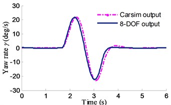
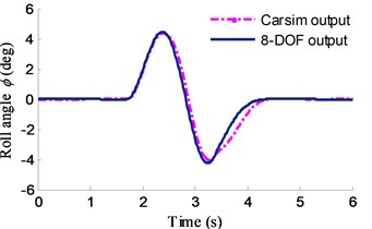
To verify the effectiveness of the 8-DOF nonlinear vehicle model with ME-Wheel and predictive scheme of PLTR, the steering wheel angle of the “Sine” similar with the lane change maneuver (open loop), which applied to the vehicle is shown in Fig. 17. The vehicle initial velocity is 16.7 m/s and maximum steering input to the ME-Wheel is ±0.1 rad. Fig. 18 illustrates the yaw rate and roll angle response of 8-DOF model and Carsim model.
It can be found from Fig. 18 that the difference values in both of yaw and roll motion comparisons at low speed are not significant. Fig. 19 shows the simulation results comparing the actual LTR by Eq. (22) and the estimated LTR by Eq. (23) during a lane change maneuver. The maximum error of the two different methods is about 12 % in the peak.
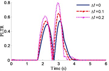
Fig. 20 shows the estimated PLTR by different preview timeunder a same steering input. As can be seen the preview time 0.1 shows a time advance (about 0.2 s) compared with the LTR ( 0) and the maximum error is about 15 % in the peak value. However, when 0.2, LTR will large than 40 %. Considering the actual situation, the value of is set 0.1.
Fig. 17Steer angle input (Nominal steering gear ratios is 20)
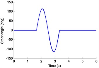
Fig. 18Yaw rare and roll angle response comparisons
a)
b)
Fig. 19Result of the LTR comparisons
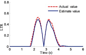
Fig. 20PLTR comparisons by different preview time (Δt)
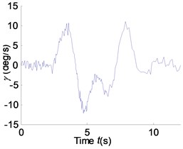
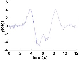
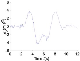
For the rollover warning system by sensor measurements always with observation noise, 5 percent of Gaussian random white noise is added. The Kalman filter is used to eliminate measurement noise and double lane change (DLC) simulation is carried out in MatLab to evaluate the robustness of the rollover warning system. The Yaw rate, roll angle and lateral acceleration response with observation noise are shown in Fig. 21. The results of PLTR with noise is shown in Fig. 22 compared with simulation results without states filter.
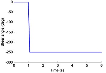
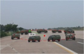
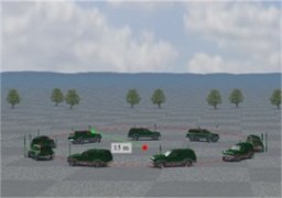
It is clear from Fig. 22 that the PLTR is unstable when the warning system without states filter and a predictive index has a filter is very necessary. The proposed vehicle model was also verified by a real vehicle testing. Steering wheel angle of step input test is used here for the inspection of the vehicle model prediction abilities of the 8-DOF with ME-wheels. The size of the step angle is 250 deg, which is shown in Fig. 23. The test results and simulation animations of the steady turning trajectory and radius are shown in Fig. 24(a), (b).
Fig. 21Yaw rate, roll angle and lateral acceleration response with measurement noise
a)
b)
c)
Fig. 22PLTR response comparison with measurement noise
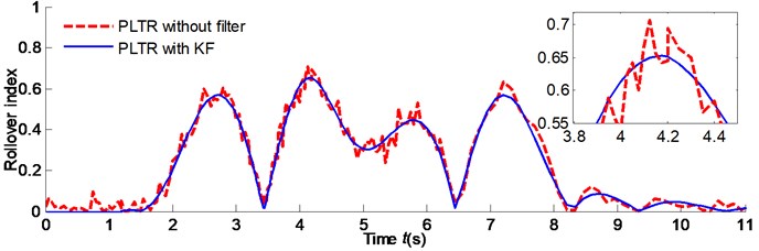
Fig. 23Steering wheel angle step input test
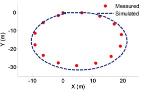
It can be found that the difference in both values of steady turning trajectory and radius (Fig. 24(a), (b)) by test and Carsim simulation are not very significant. Note that, the designed 8-DOF vehicle model is effective compared with the Carsim outputs and test results and the simulation and testing results can prove that the designed 8-DOF nonlinear vehicle model with ME-Wheel can be used as the simulated model of the off-road vehicle.
Fig. 24a) Test results of the steady turning trajectory and radius, b) simulation animations of the steady turning trajectory and radius, c) steady turning trajectory comparison
a)
b)
c)
4.2. YSC and RSC simulation and analysis
The proposed integrated (YSC+RSC) stability controller is implemented under the Simulink platform. To analysis and evaluate the proposed integrated control scheme, the algorithms of YSC and RSC are also established, respectively. And all the algorithms are evaluated through the vehicle simulation. The maneuvers of Lane change and Fishhook are tested which are conducted on the high adhesion coefficient of 0.85, respectively.
4.2.1. Lane change maneuver test
The steer angle which applied to the simulated model is shown in Fig. 17 and the initial speed is 80 km/h. To evaluate the proposed rollover evaluation index of PLTR in RSC, the compared controller is the same as Fuzzy PID except that rollover index PLTR is calculated when 0 (). The roll angle response comparison based on same RSC control methods with two kinds of rollover evaluation index of LTR and PLTR is shown in Fig. 25.
Fig. 25Roll angle response comparisons of RSC using PLTR and LTR
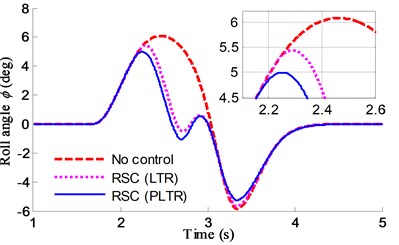
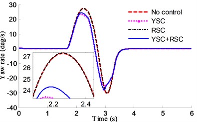
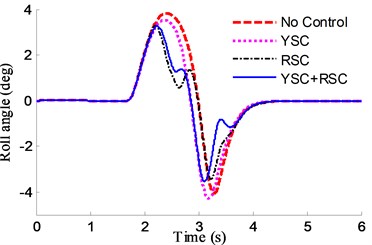
It is clear from Fig. 25 that reduction in peak value of roll angle in case of only RSC based on Fuzzy PID is more than 10 %. It also can be found that the controller using rollover evaluation index of PLTR is better than the LTR for rollover resistance. The yaw rate and roll angle response comparison based on different control methods is shown in Fig. 26.
Fig. 26Lane change maneuver test by different controllers: a) yaw rate, b) roll angle
a)
b)
As is shown in Fig. 26(b), reduction in peak value of roll angle in case of RSC and YSC+RSC with rollover evaluation index of PLTR control is more than 20 %, and about 5 % in case of YSC. It also can be found in Fig. 26(a) that the yaw values of YSC+RSC and YSC controllers are better than the values of RSC controller, which means the proposed integrated controller has advantages in sideslip and rollover control. The brake torque of 4 wheels is shown in Fig. 27.
It is noted that the control scheme proposed here can keep the vehicle cornering more stable than the uncontrolled vehicle. The decrease in vehicle rolling moment is bigger than that in YSC control case for the bigger brake force to guarantee the rollover index in a designed range.
4.2.2. Fishhook test
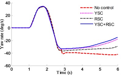
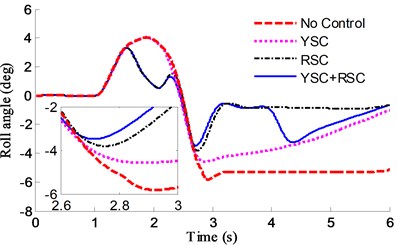
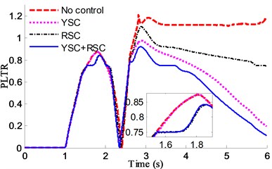
A critical maneuver of Fishhook test has also been generated. The steer angle for the fishhook maneuver is shown in Fig. 28. The initial speed is 50 km/h. The yaw and roll response and the PLTR comparison based on different controllers are shown in Fig. 29 and Fig. 30.
Fig. 27Brake target of 4 wheels by different controllers
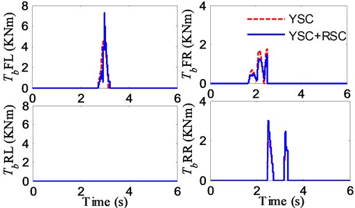
Fig. 28Steer angle input for fishhook maneuver
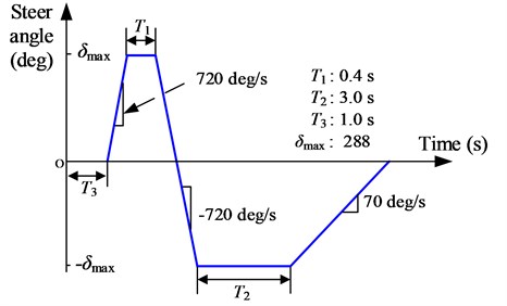
Fig. 29Fishhook test by different controllers: a) yaw rate, b) roll angle
a)
b)
It can be found in Fig. 29(b) that reduction in peak value of roll angle in case of RSC and YSC+RSC with rollover evaluation index of PLTR control is more than 100 %, and about 50 % in case of YSC, it also can be found in Fig. 29(a) that the yaw values of YSC+RSC are the smallest in the 3 comparison controllers, which means the integrated controller can earlier adjust the active suspension in rollover control and the active braking in side slip control.
It can be found from Fig. 30 that both values of PLTR by different controllers are better than that without control and the value of PLTR by YSC+RSC controller based on fuzzy PID is the smallest and the best compared with the others.
Fig. 30Roll index of PLTR comparisons in fishhook by different controllers
It is noted that though the cornering is fast and the vehicle speed is high, the control scheme proposed here can still keep the vehicle in stably while the uncontrolled vehicle will lose stability rapidly and drift or rollover.
From the simulation result, it is clear that the integrated controller is successfully designed and the proposed YSC+RSC based on Fuzzy-PID with rollover evaluation index of PLTR shows good control ability and performance.
5. Conclusions
In this paper, an integrated control of yaw and roll based on Fuzzy PID for an off-road vehicle with ME-Wheel is designed. The control system is achieved through an 8-DOF nonlinear vehicle model and a PLTR index. The results are summarized as follows.
1) The 8-DOF nonlinear vehicle model is built up and the results show that the model is effective compared with the Carsim outputs and test results.
2) Based on brush modeling theory, longitudinal and steady-state cornering mixed model of ME-Wheel are established and tested.
3) The rollover index of PLTR can provide a time-advanced measurement of rollover prediction and its accuracy is verified by virtual tests.
4) The integrated YSC+RSC controller based on Fuzzy-PID with rollover evaluation index of PLTR shows good control performance and improve the rollover and yaw stability of the vehicle, which can prevent rollover happening under emergency.
References
-
Aripin M. K., Sam Y. M., Danapalasingam K. A., et al. A review of active yaw control system for vehicle handling and stability enhancement. International Journal of Vehicular Technology, Vol. 2014, 2014, p. 437515.
-
Park M., Lee S., Kim M., et al. Integrated differential braking and electric power steering control for advanced lane-change assist systems. Proceedings of the Institution of Mechanical Engineers, Part D Journal of Automobile Engineering, Vol. 229, Issue 7, 2014, p. 924-943.
-
Yang X., Wang Z., Peng W. Coordinated control of AFS and DYC for vehicle handling and stability based on optimal guaranteed cost theory. Vehicle System Dynamics, Vol. 47, Issue 1, 2009, p. 57-79.
-
Wu J., Cheng S., Liu B., et al. A human-machine-cooperative-driving controller based on AFS and DYC for vehicle dynamic stability. Energies, Vol. 10, Issue 11, 2017, p. 1737.
-
Li L., Ran X., Wu K., et al. A novel fuzzy logic correctional algorithm for traction control systems on uneven low-friction road conditions. Vehicle System Dynamics, Vol. 53, Issue 6, 2015, p. 711-733.
-
Wu J., Wang X., Li L., et al. Hierarchical control strategy with battery aging consideration for hybrid electric vehicle regenerative braking control. Energy, Vol. 145, 2018, p. 301-312.
-
Engineer Y. S. C., Shimada K., Tomari T. Improvement of vehicle maneuverability by direct yaw moment control. Vehicle System Dynamics, Vol. 22, Issue 5, 1993, p. 465-481.
-
Raksincharoensak P., Nagai T. Direct yaw moment control system based on driver behaviour recognition. Vehicle System Dynamics, Vol. 46, Issue 1, 2008, p. 911-921.
-
Li L., Lu Y., Wang R., et al. A 3-dimentional dynamics control framework of vehicle lateral stability and rollover prevention via active braking with MPC. IEEE Transactions on Industrial Electronics, Vol. 99, Issue 6, 2016, p. 1-12.
-
Chen B.-C., Peng H. Differential-braking-based rollover prevention for sport utility vehicles with human-in-the-loop evaluations. Vehicle System Dynamics, Vol. 36, Issues 4-5, 2001, p. 359-389.
-
Solmaz S. Switched stable control design methodology applied to vehicle rollover prevention based on switched suspension settings. IET Control Theory and Applications, Vol. 5, Issue 9, 2011, p. 1104-1112.
-
Kamal M., Shim T. Development of active suspension control for combined handling and rollover propensity enhancement. SAE Technical Paper, 2007.
-
Yim S., Park Y., Yi K. Design of active suspension and electronic stability program for rollover prevention. International Journal of Automotive Technology, Vol. 11, Issue 2, 2010, p. 147-153.
-
Yim S. Design of a robust controller for rollover prevention with active suspension and differential braking. Journal of Mechanical Science and Technology, Vol. 26, Issue 1, 2012, p. 213-222.
-
Imine H. Rollover risk prediction of heavy vehicle in interaction with infrastructure. International Journal of Heavy Vehicle Systems, Vol. 14, Issue 3, 2007, p. 294-307.
-
Li H., Zhao Y., Wang H., et al. Design of an improved predictive LTR for rollover warning systems. Journal of the Brazilian Society of Mechanical Sciences and Engineering, Vol. 39, Issue 10, 2017, p. 3779-3791.
-
Rajamani R. Vehicle Dynamics and Control. 2nd ed., Springer-Verlag, New York, NY, USA, 2012.
-
Chen K., Guo X., Pei X. Rollover warning of commercial vehicles based on multiple condition matching. China Mechanical Engineering, Vol. 27, Issue 20, 2016, p. 2822-2827.
-
Johansen T. A. Integration of vehicle yaw stabilization and rollover prevention through nonlinear hierarchical control allocation. Vehicle System Dynamics, Vol. 52, Issue 12, 2014, p. 1607-1621.
-
Cao J., Jing L., Guo K., et al. Study on integrated control of vehicle yaw and rollover stability using nonlinear prediction model. Mathematical Problems in Engineering, Vol. 2013, 2013, p. 643548.
-
Zhao Y., Li H., Lin F., et al. Estimation of road friction coefficient in different road conditions based on vehicle braking dynamics. Chinese Journal of Mechanical Engineering, Vol. 30, Issue 4, 2017, p. 982-990.
-
Li L., Yang K., Jia G., et al. Comprehensive tire-road friction coefficient estimation based on signal fusion method under complex maneuvering operations. Mechanical Systems and Signal Processing, Vol. 56, 2015, p. 259-276.
-
Li H., Zhao Y., Lin F., et al. Nonlinear dynamics modeling and rollover control of an off-road vehicle with mechanical elastic wheel. Journal of the Brazilian Society of Mechanical Sciences and Engineering, Vol. 40, Issue 2, 2018, p. 51.
-
Yang X., Li H., Gao J., et al. Parameter estimation for tractor- semitrailer vehicle based on recursive least square method. Journal of Kunming University of Science and Technology, Vol. 39, Issue 3, 2014, p. 43-49.
Cited by
About this article

This work was supported by the National Natural Science Foundation of China (Grant No. 11672127), the Major Exploration Project of the General Armaments Department of China (Grant No. NHAl3002), the Postgraduate Research and Practice Innovation Program of Jiangsu Province (Grant No. KYCX17_0240), and the Fundamental Research Funds for the Central Universities (Grant No. NP2016412, NP2018403, NT2018002). The author greatly appreciated the financial support.
