DC modulation controller parameters tuning based on improved multi-signal Prony algorithm

Su, Hongsheng; Zhu, Zongkong

Journal of Vibroengineering

Browse Journal

Submit article

Published: 30 September 2015

Check for updates

DC modulation controller parameters tuning based on improved multi-signal Prony algorithm

Hongsheng Su¹

Zongkong Zhu²

^{1, 2}School of Automation and Electrical Engineering, Lanzhou Jiaotong University, Lanzhou 730070, P. R. China

Corresponding Author:

Hongsheng Su

Cite the article Download PDF

Downloads 1196

Abstract

To aim at the puzzle of DC modulation controller parameters tuning in large-scale AC/DC interconnected power systems, in this paper a multi-signal Prony algorithm is proposed which can simultaneously extracts oscillation modes from multiple signals compared with traditional Prony analysis method. In the algorithm, current setting value increment at rectifier side serves as system input, and AC liaison transmission line active power increment acts as the resulting output under consideration of systems initialization state. Through the improved multi-signal Prony identification on the output time-domain response data under specified input, an equivalent linear model with order reduced is obtained. Based on the identified results, the adjustments are then implemented on the controller parameters using the pole placement method. Through theoretical analysis and IEEE four generators system tests, the simulation results show that to add the DC modulation controller with parameters tuned by the improved Prony algorithm can significantly increase the oscillation damping of AC/DC interconnected systems, and improve the systems operation stability.

1. Introduction

With the expansion of AC/DC power grids interconnection, the size of modern power systems is becoming larger and larger, and the structure of which is becoming more and more complex, which results in a higher requirement on the analysis and control of systems. The analysis and suppression of inter-area low frequency oscillation in AC/DC interconnected power grids now has already become a more difficult and important puzzle [1-3]. The traditional methods such as eigen-values and frequency domain analysis require a complete detailed precise mathematical model, but usually to do so is a difficult task. In another hand, the modern identification technology can identify the system model reduced not rely on the mathematical model of each component [4]. The Prony identification can estimate the system oscillation modes through analysis on the measured data, which include the oscillation frequency, damping, amplitude and phase, and etc. Further, the identification can directly obtain the characteristic roots of systems, and the residue of transfer function, and other information. And thus, it can avoid having to create an accurate model of the system and solve high-order matrix. Hence, it is particularly suitable for analysis on power systems response signal and the design of control systems [5, 6].

In recent years, with the development of high voltage direct current (HVDC) transmission technology in China, there would be more than 20 ultra HVDC lines to be put into operation by 2020 [7]. In view of its fast response, and flexible control on the HVDC transmission systems, and as well as strong modulation capacity, DC modulation controller can be used to modulate the power of DC transmission line. This is thought to be one of the most effective means to suppress the inter-area low frequency oscillation of interconnect power grids [8]. The relative investigations have shown that the selection of DC modulation signal, and load model, and the modulator parameters are the key elements to influence modulation effects. In [9] trajectory sensitivity is applied to analyze the DC modulator parameters, and the results are verified using a four-generator system. But the method needs to calculate systems gradient information, and it is difficult for the large-scale AC/DC hybrid systems. In [10] modulator parameters are optimized by genetic algorithm (GA). Due to its stronger randomness of optimization algorithm, there are some shortcomings existing of slow convergence. In [11] Prony method is proposed to identify the system transfer function very convenient, and possesses higher accuracy than the test signal method.

Prony analysis possesses many applications in AC systems such as the design of excitation regulator and PSS, but there have been little attentions in AC/DC hybrid transmission systems. In addition, Prony methods always assume that the system is single output, and each signal is analyzed, independently, which often results in estimates conflicting in frequency and damping due to noise effects [12]. And so it is difficult to determine which signal identification result is most reasonable and accurate. In [13], an extended Prony algebraic interpolation scheme is proposed to find the nearest analytic function of algebraic interpolant on an equispaced grid, and the interpolation errors of the method are much lower compared with the classic schemes on equispaced grids, which can be effectively exploited for analytic interpolation of noisy or defected signals. But the method based on the nearest algebraic interpolant does not suppress the Runge phenomenon, the calculation will increase and produce more serious error accumulation such that the stability can not be guaranteed. In [14] wide area measurement system (WAMS) can obtain the global oscillation information, and provide full support to suppress the inter-area low frequency oscillation, which make the multi-signal combined identification possible. In this paper, on the basis of WAMS, multi-signal is firstly introduced into Prony algorithm for identification of low frequency oscillation in AC/DC hybrid systems, and wavelet transform is then applied to eliminate the signal noise. Secondly, multi signals sample function matrix is established and singular value decomposed-total least square (SVD-TLS) method is used to determine the order of signal. Thirdly, the improved multi-signal Prony algorithm is proposed to identify the system output characteristics, and transfer function is then obtained, and then combining with the pole placement method to adjust the DC modulation controller parameters. Finally, the applicability and superiority of the proposed method are verified through the IEEE four-generator system.

2. System transfer function identification based on Prony algorithm

2.1. Traditional Prony algorithm

Prony algorithm can fit several exponential functions into a signal though linear combination, and which is shown by [15]:

1

\hat{x} (n) = \sum_{i = 1}^{p} b_{i} z_{i}^{n} = A_{i} e x p (j θ_{i}) e x p [(α_{i} + j 2 π f_{i}) Δ t], n = 0, 1, \dots, N - 1,

where $\hat{x} (n)$ expresses the estimated value of the $n$ th sampling point, and $N$ takes integer, and $p$ expresses the number of exponential functions and takes integer, and $A_{i}$ is the amplitude of signal trace, and $θ_{i}$ is the corresponding phase (unit: rad), and $α_{i}$ represents the attenuation factor, and $f_{i}$ means the oscillation frequency, and $∆ t$ is the sampling interval.

2.2. Improved Prony algorithm

Traditional Prony algorithm always assumes that the system is single output, which is not consistent with power systems of single-input and multiple-output. Due to disturbance from noise and other factors, the obtained outcome will lead to conflicting modality estimates. And so it is difficult to determine which modality estimates are accurate. In addition, since power system is a complex large system, and for large systems, the single signal analysis on system oscillation mode is limited. In order to identify system oscillation modes as much as possible, the multiple signals are introduced to extract oscillation characteristics, and fit into each output under same modality so as to improve identification accuracy, and then:

2

{\hat{x}}_{k} (n) = \sum_{i = 1}^{p} b_{k i} z_{i}^{n},

where ${\hat{x}}_{k} (n)$ presents the model of measured data, $b_{k i}$ and $z_{i}$ are both complex, and expressed by:

3

\{\begin{array}{l} b_{k i} = A_{k i} e x p (j θ_{k i}), \\ z_{i} = e x p [(α_{i} + j 2 π f_{i}) Δ t], \end{array}

where $A_{k i}$ is the amplitude of the $k$ th signal trace, and $θ_{k i}$ is its phase, $α_{i}$ , $f_{i}$ and $∆ t$ possess same implications with Eq. (1).

Now we consider the multi-signal traces, and cost function is constructed by:

4

ε = \sum_{k = 1}^{M} \sum_{n = 0}^{N - 1} {|x_{k} (n) {- \hat{x}}_{k} (n)|}^{2},

where $M$ is the total number of signal traces, and $x_{k} (n)$ is the actual value of the $k$ th signal trace, and ${\hat{x}}_{k} (n)$ is the corresponding estimated value.

Similar to single signal trace derivation process, multiple signal traces apply a set of same exponential signal to approximate multiple signals, simultaneously, and make mean squares sum of all curves minimum. According to least mean squares (LMS), we can obtain the parameters of $A_{k i}$ , $θ_{k i}$ , $α_{i}$ and $f_{i}$ [16].

${\hat{x}}_{k} (n)$ meets the recursive difference equation described by:

5

{\hat{x}}_{k} (n) = - \sum_{i = 1}^{p} a_{i} {\hat{x}}_{k} (n - i) .

Let $e (n)$ be the error between the measured data and the estimated value, and thus we have:

6

x_{k} (n) = {\hat{x}}_{k} (n) + e (n) .

Substituting Eq. (5) into Eq. (6), we obtain:

7

x_{k} (n) = - \sum_{i = 1}^{p} a_{i} {\hat{x}}_{k} (n - i) + e (n) = - \sum_{i = 1}^{p} a_{i} x_{k} (n - i) + \sum_{i = 0}^{p} a_{i} e (n - i),

a_{0} = 1, n = 0, 1, \dots, N - 1 .

Define $ε (n) = \sum_{i = 0}^{p} a_{i} e (n - i)$ , and we then have:

8

x_{k} (n) = - \sum_{i = 1}^{p} a_{i} x_{k} (n - i) + ε (n) .

Define the cost function as:

9

J (a) = \sum_{n = p}^{N - 1} {|ε (n)|}^{2} = \sum_{n = p}^{N - 1} {|\sum_{i = 0}^{p} a_{i} x_{k} (n - i)|}^{2} .

From Eq. (9), we have:

\frac{\partial J (a)}{\partial a_{i}} = 0, i = 1, 2, \dots, p .

And then we obtain:

10

\sum_{i = 0}^{p} a_{i} [\sum_{n = p_{}}^{N - 1} x_{k} (n - i) x_{k}^{*} (n - j)] = 0, j = 1, 2, . . ., p .

Improved multi-signal Prony algorithm is then described as follows.

1) To define sample function matrix by:

11

R = [\begin{matrix} r (1,0) & r (1,1) & \dots & r (1, p_{e}) \\ r (2,0) & r (2,1) & \dots & r (2, p_{e}) \\ ⋮ & ⋮ & ⋱ & ⋮ \\ r (p_{e}, 0) & r (p_{e}, 1) & \dots & r (p_{e}, p_{e}) \end{matrix}],

where:

12

r (i, j) = \sum_{k = 1}^{M} \sum_{n = p_{}}^{N - 1} x_{k} (n - i) x_{k}^{*} (n - j), i, j = 0, 1, \dots, p,

and $M$ expresses the number of signal traces, and $p_{e}$ is the order of prediction model, and $x_{k} (i)$ is the $i$ th sample point of the $k$ th signal.

2) To obtain $a$ by:

13

[\begin{matrix} r (1,0) & r (1,1) & \dots & r (1, p_{e}) \\ r (2,0) & r (2,1) & \dots & r (2, p_{e}) \\ ⋮ & ⋮ & ⋱ & ⋮ \\ r (p_{e}, 0) & r (p_{e}, 1) & \dots & r (p_{e}, p_{e}) \end{matrix}] [\begin{matrix} 1 \\ a_{1} \\ ⋮ \\ a_{p} \end{matrix}] = [\begin{matrix} ε_{p} \\ 0 \\ ⋮ \\ 0 \end{matrix}] .

The effective rank $p$ of matrix $R$ , and as well as the coefficients $a_{1}$ , $a_{2}$ ,…, $a_{p}$ of corresponding oscillation pattern can be determined using SVD-TLS algorithm

3) The eigenvalues of the polynomial $1 + a_{1} z^{- 1} + a_{2} z^{- 2} + . . . + a_{p} z^{- p} =$ 0 can be calculated based on the $a_{1}$ , $a_{2}$ ..., $a_{p}$ . And then we can obtain by the following recursive formula:

14

{\hat{x}}_{k} (n) = - \sum_{i = 1}^{p} a_{i} {\hat{x}}_{k} (n - i),

where ${\hat{x}}_{k} (0) = x_{k} (0)$ .

4) To calculate the parameters $b_{k i}$ according to the following equation:

15

[\begin{matrix} 1 & 1 & \dots & 1 \\ z_{1} & z_{2} & \dots & z_{p} \\ ⋮ & ⋮ & ⋱ & ⋮ \\ z_{1}^{N - 1} & z_{2}^{N - 1} & \dots & z_{p}^{N - 1} \end{matrix}] [\begin{matrix} b_{k 1} \\ b_{k 2} \\ ⋮ \\ b_{k p} \end{matrix}] = [\begin{matrix} {\hat{x}}_{k} (0) \\ {\hat{x}}_{k} (1) \\ ⋮ \\ {\hat{x}}_{k} (N_{k} - 1) \end{matrix}] .

5) To calculate frequency, and the attenuation factor, and the amplitude and phase of each signal as follows:

16

\{\begin{array}{l} A_{k i} = |b_{k i}|, \\ θ_{k i} = \frac{a r c t a n [\frac{I m (b_{k i})}{R e (b_{k i})}]}{2 π Δ t}, \\ α_{i} = \frac{l n |z_{i}|}{Δ t}, \\ f_{i} = \frac{a r c t a n [\frac{I m (z_{i})}{R e (z_{i})}]}{2 π Δ t}, \end{array}

where $k$ denotes the $k$ th signal, and $i$ denotes the $i$ th component.

2.3. System transfer function identification

System model is shown in Fig. 1, where $G (s)$ expresses system transfer function, and $u (t)$ is system excitation signal, and $y (t)$ is system output, and $y_{e x} (t)$ is system stimulus-response, and $y_{0} (t)$ is the initial state of system.

Fig. 1System model

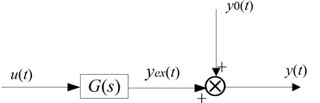
Pole residue form of $G (s)$ and $Y_{0} (s)$ can be expressed by:

17

Y_{0} (s) = \sum_{i = 1}^{n} \frac{A_{i}}{s - λ_{i}},

18

G (s) = \sum_{i = 1}^{n} \frac{R_{i}}{s - λ_{i}},

where $n$ is the order of transfer function, and $λ_{i}$ is the eigenvalues of system, and $R_{i}$ is the residue of transfer function, and $A_{i}$ is the residue of initial state.

The aim to identify transfer function and initial state of system is to find the estimate values of $λ_{i}$ , $R_{i}$ , $A_{i}$ and $n$ , such that the model output as close as possible to the actual output [17].

Let us assume that $U (s)$ is composed of limited entry delay factor $c_{i}$ and eigenvalues $D_{j}$ , and then:

19

U (s) = \frac{(c_{0} + c_{1} e^{- s D_{1}} + c_{2} e^{- s D_{2}} + \dots + c_{k} e^{- s D_{k}})}{s - λ_{n + 1}}, i, j = 0, 1, \dots, k .

Consider the effect of the input signal $U (s)$ , the output $Y (s)$ should contain the modes caused by the input signal and system itself, which can be expressed by:

20

Y (s) = Y_{0} (s) + Y_{e x} (s)

= (c_{0} + c_{1} e^{- s D_{1}} + c_{2} e^{- s D_{2}} + \dots + c_{k} e^{- s D_{k}}) \sum_{i = 1}^{n} \frac{R_{i}}{(s - λ_{n + 1}) (s - λ_{i})} + \sum_{i = 1}^{n} \frac{A_{i}}{s - λ_{i}} .

By partial fraction, the above formula can be expanded by:

21

Y (s) = (c_{0} + c_{1} e^{- s D_{1}} + c_{2} e^{- s D_{2}} + \dots + c_{k} e^{- s D_{k}}) [\frac{Q_{n + 1}}{s - λ_{n + 1}} + \sum_{i = 1}^{n} \frac{Q_{i}}{s - λ_{i}}],

where:

22

Q_{i} = \frac{R_{i}}{λ_{i} - λ_{n + 1}}, Q_{n + 1} = - \sum_{i = 1}^{n} Q_{i} .

Since $t \geq D_{k}$ , so that $D_{0} = 0$ , then $y (t)$ is:

23

y (t) = Q_{1} (\sum_{i = 0}^{k} ‍ c_{i} e^{- λ_{1} D_{i}}) e^{λ_{1} t} + Q_{2} (\sum_{i = 0}^{k} ‍ c_{i} e^{- λ_{2} D_{i}}) e^{λ_{2} t}

+ \dots + Q_{n + 1} (\sum_{i = 0}^{k} ‍ c_{i} e^{- λ_{n + 1} D_{i}}) e^{λ_{n + 1} t} .

Since $t$ is bound to be greater than $D_{k}$ , the above formula can not be directly analyzed by Prony method. Let $τ = t - D_{k}$ , and $v (τ) = y (τ + D_{k})$ , the above equation then can be written by:

24

v (τ) = \sum_{j = 1}^{n + 1} B_{j} e^{λ_{j} τ} .

Consider the non-zero initial state conditions [18], and then have further Prony identification, we will obtain the residue of transfer function:

25

B_{j} = Q_{j} (\sum_{i = 0}^{k} ‍ c_{i} e^{- λ_{j} (D_{k} - D_{i})}) + A_{j} e^{λ_{i} D_{k}}, j = 1, 2, . . ., n + 1 .

Substituting the above formula into Eq. (22), the transfer function residue then is:

26

R_{j} = \frac{B_{j} (λ_{j} - λ_{n + 1})}{\sum_{i = 0}^{k} ‍ c_{i} e^{λ_{j} (D_{k} - D_{i})}} .

$B_{j}$ and $λ_{j}$ in Eq. (26) can be obtained from Eq. (24) using Prony analysis, $c_{i}$ , $D_{j}$ and $λ_{n + 1}$ are obtained based on the input. Therefore, the input in Eq. (19) will be applied into the real system, then through the results of improved multi-signal Prony analysis and further calculation, system transfer function can be obtained.

3. AC/DC power system model and HVDC additional damping control

3.1. Principle of AC/DC power system interaction

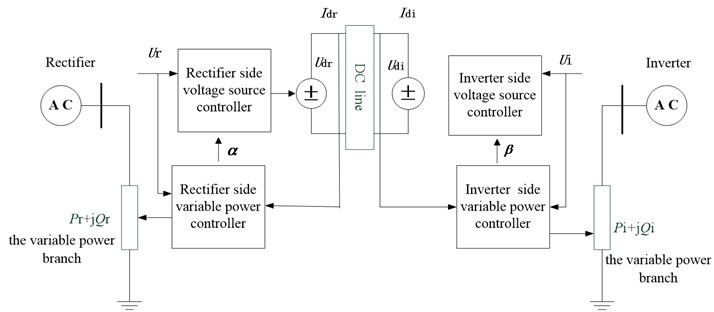
In the AC/DC power system simulation, to reflect the impact of DC system on AC system stability more accurately, here we apply more accurate HVDC quasi-steady-state model in [1]. The AC system and DC system are independently solved, and AC system and DC system interacts as shown in Fig. 2. The impact of DC system on AC system may be seen as a change of load or voltage source. HVDC quick adjustment feature is implemented by changing the power of the variable power branch [19].

Fig. 2Diagram of interaction of AC/DC system

3.2. DC modulation controller model

DC modulation controller model is used in [1]. In this paper, it is generally believed that the current control is fast, and constant current control can prevent a substantial change in current, limiting the over-current and preventing from the converter overload. And constant extinction angle control can avoid commutation failure at inverter side, and maintain the DC voltage at a high level, so we adopt the operation mode of constant current in rectifier side, and constant extinction angle in inverter side. The constant current controller and DC modulation model are shown in Fig. 3.

Fig. 3DC modulation controller model

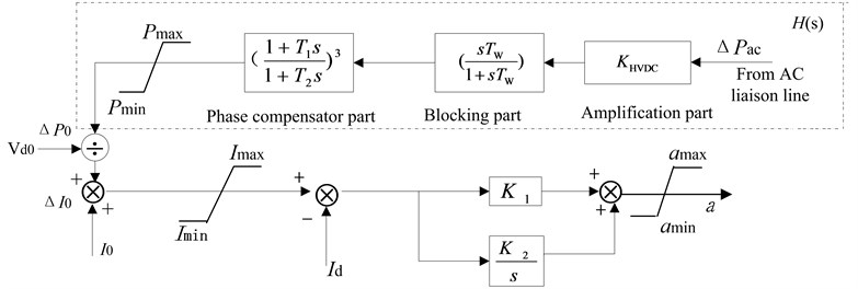
In Fig. 3, $I_{d}$ and $I_{0}$ denote the input signal of constant current controller and the current setting value of rectifier, respectively. $T_{W}$ denotes the time constant of blocking part, $T_{1}$ and $T_{2}$ denote the time constant of lead-lag parts, $K_{H V D C}$ denotes the gain coefficient, subscript max and min denote the upper and lower limits of the corresponding variable amplitude.

The active power increment $Δ P_{a c}$ of AC liaison transmission lines is set as the input signal of DC modulator, and through the measurement, blocking part and phase compensator composed by a series of lead-lag parts and amplification part to synthesize, eventually outputs additional power control signal through clipper. While the signal is overlapped with the power control command signal, through the output of constant current regulator in pole control unit and changes the trigger angle $α$ command of rectifier, which is sent to the valve control units to control the DC power output. By adjusting the transmission power of DC lines, which can rapidly absorb and compensate for excess power or shortfall power connected thereto AC system, so that the power can reach equilibrium, and reduce the transmission pressure of AC transmission system. Serving to strengthen the effect of AC system damping and improving AC/DC interconnected system stability [20].

3.3. DC modulation controller design

In parallel AC and DC power transmission systems, The DC current setting value increment $Δ I_{0}$ is selected as the control variable, and the active power increment $Δ P_{a c}$ of AC liaison lines is set as the controlled variable. Assuming that identified system transfer function is $G (s)$ , the controller transfer function is $H (s) .$ And $Δ P_{a c}$ is introduced as a feedback variable, the closed-loop system is shown in Fig. 4.

Fig. 4System closed-loop block diagram

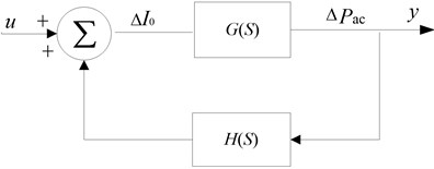
From Fig. 4, the system transfer function can be obtained by:

27

G_{c} (s) = \frac{G (s)}{1 - G (s) H (s)} .

Assuming that after adding the feedback compensation parts, the new dominant pole of closed-loop system is $s_{d}$ , and the eigenvalues of system is moved to the location $λ_{0}$ . Then $λ_{0}$ must satisfy the characteristic equation $1 - G (s) H (s) =$ 0 of the closed-loop system, so we can get $H (s_{d}) = 1 / G (s_{d})$ , which can be written in the form of amplitude and phase angle below:

28

|H (s_{d})| = \frac{1}{|G (s_{d})|}, a r g (H (s_{d})) = - a r g (G (s_{d})) .

Therefore, through the amplitude and phase angle values at $s = s_{d}$ of the identified system transfer function, we can obtain the amplitude and phase angle of DC modulation controller at $λ_{0}$ , so that the new pole location will be selected to meet the specific damping ratio, then take advantage of lead-lag links to meet phase compensation. Finally, we can select the gain to meet the amplitude equation.

3.4. Stability analysis with DC modulation controller

According to linear control theory [21], the characteristic polynomial of the $G (s)$ can be described as:

29

α_{G} (s) ≜ {α_{0} s}^{n} + α_{1} s^{n - 1} + α s^{n - 2} + \dots + α_{n - 1} s + α_{n} .

And then the poles of $G (s)$ is denoted as the roots of the characteristic equation $α_{G} (s) =$ 0. If all the ploes is located on the left side of the imaginary axis in the complex plane, namely, they are the negative real numbers or possess the negative real parts, and then the system characterized by $G (s)$ can be said stable, and instable if there is a ploe located in imaginary axis or the right side of the imaginary axis in the complex plane otherwise.

The introduction of state feedback $H (s)$ changes the system transfer function, namely, $G (s)$ is converted to $G_{c} (s)$ , and characteristic eauation $α_{G} (s)$ to $α_{G c} (s)$ , correspondingly, the roots of the characteristic eauation is changed. In other words, in system synthesis, to obtain desired properties we can apply diverse feedback matrix $H (s)$ to change the location of the zeros and ploes, since they possess significant inflence on system behavior. In this paper, from Fig. 3, we can select suitable $H (s)$ to change the location of the poles, such that the expected dynamical properties can be acquired.

4. Examples

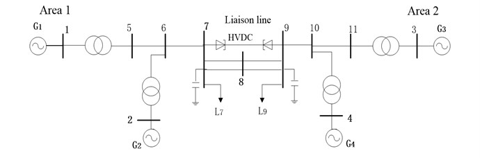
Fig. 5 shows the structure of IEEE four-generator system, and system parameters can be found in [1], where the rated power of DC line is 1000 MW, and the rated voltage of AC line is 230 KV, the rated capacity of each generator is 900 MWA, rated voltage is 20 KV, and generator model includes the excitation system and the speed control system, and the load uses constant resistance, and as well as two terminals HVDC systems adopts quasi-steady-state model, wherein the left side is the rectifier station, and the right one is the inverter station. The control system adopts the operation mode of constant current in rectifier side and constant extinction angle in inverter side. DC modulation controller is attached to the side of the rectifier side of the verification system. DC modulation controller is as shown in Fig. 3.

Fig. 5IEEE four-generator test system

4.1. Modal identification based on improved multi-signal algorithm

In this example, three-phase short circuit fault occurs in the bus 7-side starting at the 1.0 s, and is cleared at five cycle later. Each generator power angle curve closely related to the electromechanical oscillations is selected, and the Prony modal identification is adopted mentioned in Section 2.1. In this paper, the relative power angle of each generator and AC liaison line active power are set as the identification signals, and the generator G1 is considered as reference machine. Table 1 and Table 2 are respectively single signal and improved multi-signal algorithm for each generator relative power angle identification results.

Seen from Table 1, when adopts the signals of different units each time can identify the dominant mode of system accurately, namely, the inter-area oscillation mode. However, for the identification of local oscillation modes, the identification results are quite different. In model model 2, and model 3, and as well as model 4, applying the signals of same area can get different estimate results even contradictory results, which makes the choice of frequency and damping ratio of local oscillation modes become very difficult, and it is not conducive to have further identification. However, in Table 2, when using multiple signals can identify all oscillation modes, and the results are more accurate than the ones of single signal.

Table 1Each generator power angle identification results based on single signal Prony algorithm

Identification signals and parameters		Mode 1	Mode 2	Mode 3	Mode 4
$δ_{21}$	$f$ / Hz	0.575	1.107	1.253	0.837
$δ_{21}$	Damping ratio	0.016	0.062	–0.001	0.300
$δ_{31}$	$f$ / Hz	0.577	0.976	1.285	1.767
$δ_{31}$	Damping ratio	0.016	0.135	0.035	0.046
$δ_{41}$	$f$ / Hz	0.575	0.866	1.110	1.110
$δ_{41}$	Damping ratio	0.016	0.036	0.120	0.120
Comprehensive analysis	$f$ / Hz	0.575	0.913	1.110	–
Comprehensive analysis	Damping ratio	0.016	0.175	0.120	–

Table 2Generator power angle identification results based on improved multi-signal Prony algorithm

Identification signals and parameters	Mode 1	Mode 2	Mode 3	Mode 4
$f$ / Hz	0.575	0.983	1.167	1.643
Damping ratio	0.016	0.054	0.125	0.084

4.2. System transfer function identification

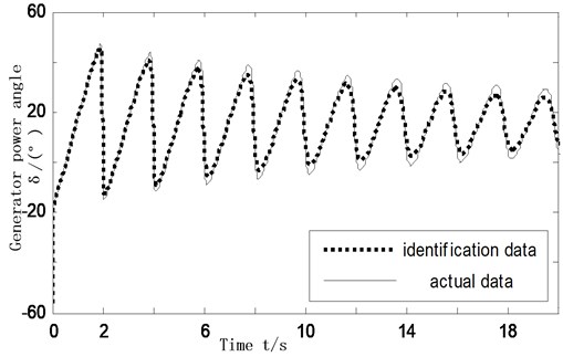
The input signal of DC modulation controller is active power increment of AC liaison line between the two regions, and system transfer function is identified in accordance with Section 2.2. The current setting of DC side adds an excitation $Δ u$ , and carries on the Prony analysis, we then obtain the transfer function from DC line at rectifier side current setting to AC liaison line active power. Table 3 shows the system initial state and reduced order transfer function based on improved multi-signal Prony algorithm identification. System output curves fitting results are shown in Fig. 6.

Table 3Order transfer function and initial state of Δu→ΔPac

$n$	$λ_{i}$	$A_{i}$	$R_{i}$
1	–9.158	0.0030	1.2328-j0.0001
2	–0.0561+j3.5101	–0.0046+j0.0162	2.1245+j3.1360
3	–0.0561-j3.5101	–0.0046-j0.0162	2.1245-j3.1360
4	–0.1815+j5.6490	–0.0015+j0.0031	0.8405+j1.3267
5	–0.1815-j5.6490	–0.0015-j0.0031	0.8405-j1.3267
6	–0.5865+j6.1839	0.0001+j0.0205	0.2175+j0.5033
7	–0.5865-j6.1839	0.0001-j0.0205	0.2175-j0.5033
8	–0.4812+j7.0375	–0.0037+j0.0007	0.2096+j0.1741
9	–0.4812-j7.0375	–0.0037-j0.0007	0.2096-j0.1741
10	–1.2486+j10.2399	0.0012+j0.0046	0.3876+j2.9004
11	–1.2486-j10.2399	0.0012-j0.0046	0.3876-j2.9004

From the analysis of Table 3, eigenvalues (–0.0561±j3.5101) and (–0.1815±j5.6490) show the mode of the system inter-area low frequency oscillation, damping ratio is small, so attenuation is slow, while the former residue is larger than that of the latter, therefore the former is system dominant oscillation mode. Additional DC modulation controller to form a closed-loop system, using the pole placement method and the damping ratio of system dominant mode will be increased to 0.15, the dominant eigenvalues is selected as 0.485±j3.20. The corresponding oscillation frequency is 0.51 Hz, and then obtain amplitude and phase of controller, which are respectively 6.28 and 113.04 deg.

According to DC modulation controller model in Fig. 3, the transfer function of DC modulation controller is shown by:

30

H (s) = \frac{K s T_{W} (1 + s T_{1})^{3}}{{(1 + T}_{W}) (1 + s T_{2})^{3}},

where $T_{w}$ is blocking time constant, which has no relation with the damping property of the controller, and generally takes for 10 s, in order to meet the requirement of improving dynamic stability, power modulation amplitude can achieve 3 % to 10 % of the DC power, so the power limiting link is ±30 MW.Through the phase requirements we can calculate $T_{1}$ and $T_{2}$ , then according to the amplitude can obtain gain $K$ , the final transfer function of DC modulation controller is obtain by:

31

H (s) = \frac{K s T_{W} (1 + s T_{1})^{3}}{{(1 + T}_{W}) (1 + s T_{2})^{3}} = \frac{0.575 \times 10 s (1 + 0.634 s)^{3}}{(1 + 10 s) (1 + 0.152 s)^{3}} .

Fig. 6Identified model output data versus actual data

4.3. Simulation results

Under the condition of above fault, these three cases are simulated in time domain without DC modulation, adds the DC modulator of traditional Prony design and DC modulator designed based on improved multi-signal Prony algorithm. The power angle of generator and AC liaison line active power steady-state simulation results are shown in Figs. 7 and 8.

Fig. 7Angle swing curves of G4 refer to G1

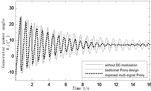
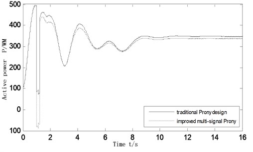
Fig. 9-10 are respectively by changing the operating mode and fault mode to verify the robustness of DC modulation controller whose parameters has been tuned. In Fig. 9, failure mode changes for the three-phase short circuit occurs in the bus 8 side, after 5 cycles fault is cleared. In Fig. 10, the L7-8 AC liaison line active power is transmitted by increased from 210 MW to 306 MW, the fault pattern is unchanged.

Fig. 8Active power oscillation curves of the inter-tie 7-8

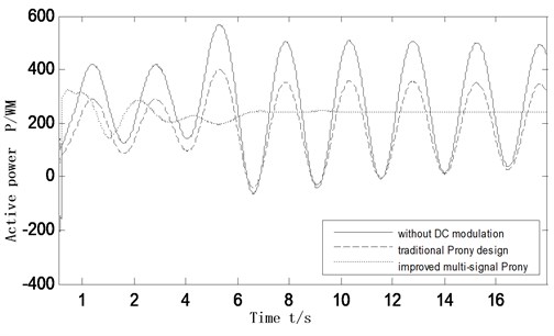
Fig. 9Active power oscillation curves of the inter-tie 7-8 as system failure mode changing

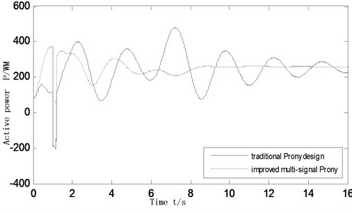
Fig. 10Active power oscillation curves of the inter-tie 7-8 as system operating mode changing

The simulation results show that the additional DC modulation controllers can indeed play a role in suppressing the inter-area low frequency oscillation, and the modulation controller parameters is the key to affecting the modulation effect. Controller designed based on the traditional single machine infinite theoretical analysis and combination of engineering practical experience can achieve a certain damping effect on power oscillation. The controller designed based on improved multi-signal Prony algorithm, then adopts pole placement and combines with the identification results to adjust controller parameters, since the identified transfer function contains information between generators and DC modulation controller, which more comprehensively consider the interaction of the whole system. The simulation shows that to add controller designed by improved algorithm makes the system can restore stability less than 10 s after a disturbance, however, the system need longer time to restore without DC modulation controller, which is not conducive to make the system have a stable operation.

Therefore system adds the controller designed by improved multi-signal Prony algorithm can improve the system damping effect greatly. It not only suppress inter-area low frequency oscillation, but also improve the stability of interconnected AC/DC system, which is consistent with the former theoretical analysis.

5. Conclusions

This paper analyzes low frequency oscillation modes of the AC/DC power transmission systems, and aims at the flaws of traditional Prony algorithm in applications, and proposes analysis method based on multiple signals Prony algorithm, and gives out the calculating process and experiment verification. The applications shows that the proposed method improves the identification accuracy and control effects and does not depend on the accurate mathematical model and parameters tuning, which can lay the foundation for the coordination optimization between controllers. DC modulation controller designed by improved multi-signal Prony algorithm can effectively improve the damping effect of the systems, and suppress inter-area low frequency oscillation so as to increase the stability of the overall system operation.

References

Prabha Kundur Power System Stability and Control. McGraw-Hill Inc., New York, 1994.

Search CrossRef
Chen Shi, Li Xingyuan, Zhao Rui Coordination research of PSS and HVDC damping control based on control sensitive factor analysis. High Voltage Engineering, Vol. 40, Issue 11, 2014, p. 3577-3583.

Search CrossRef
Blekhman I. I. Synchronization of Dynamical System. Nauka, Moscow, 1971, (in Russian).

Search CrossRef
Annissa H., Innocent Kamwa Assessment of two methods to select wide-area signals for power system damping control. IEEE Transactions on Power Systems, Vol. 23, Issue 2, 2008, p. 572-581.

Search CrossRef
Charles W. Therrien, Carlos H. Velasco An iterative Prony method for ARMA signal modeling. IEEE Transactions on Signal Processing, Vol. 43, Issue 1, 1995, p. 358-361.

Search CrossRef
Zhang Liang, Zhang Xinyan, Wang Weiqing Identification of low frequency oscillations based on improved multi-signal matrix pencil algorithm. Power System Protection and Control, Vol. 41, Issue 13, 2013, p. 26-30.

Search CrossRef
Zhu Ling, Wang Xiaoru Research of emergency DC power support strategies for large-scale power grid based on PSD-BPA. Power System Protection and Control, Vol. 41, Issue 23, 2013, p. 139-144.

Search CrossRef
Jing Yong, Hong Chao, Yang Jinbai Suppression of inter-area power oscillation in southern China power grid by HVDC modulation. Power System Technology, Vol. 29, Issue 20, 2005, p. 53-56.

Search CrossRef
Wang Changxiang, Fang Dazhong, Xue Zhenyu Parameter optimization design of DC modulation based on trajectory sensitivity analysis. Proceedings of the CSU–EPSA, Vol. 24, Issue 4, 2012, p. 30-35.

Search CrossRef
Zhu Haojun, Cai Zexiang, Liu haoming Coordinate optimization algorithm of controller in multi-infeed AC/DC power systems. Proceedings of the CSEE, Vol. 26, Issue 13, 2006, p. 7-13.

Search CrossRef
Liu Haifeng, Xu Zheng Parameters tuning of HVDC small signal modulation controllers based on test signal. Automation of Electric Power Systems, Vol. 26, Issue 21, 2002, p. 12-16.

Search CrossRef
Ma Yanfeng, Zhao Shuqiang, Liu Sen Online identification of low-frequency oscillatons based on improved multi-signal prony algorithm. Power System Technology, Vol. 31, Issue 15, 2007, p. 44-50.

Search CrossRef
Karaliene D., Navickas Z., Ciegis R., Ragulskis M. An extended Prony’s interpolation scheme on an equispaced grid. Open Mathematics, Vol. 13, Issue 31, 2015, p. 333-347.

Search CrossRef
Qi Jun, Wang Quanyuan, Cao Yijia A general Prony identification algorithm for power system transfer function. Proceedings of the CSEE, Vol. 28, Issue 28, 2008, p. 41-46.

Search CrossRef
Liu Hongchao, Li Xingyuan Study of DC damping control in AC/DC transmission systems based on Prony method. Proceedings of the CSEE, Vol. 22, Issue 7, 2002, p. 54-57.

Search CrossRef
Trudnowski D., Johnson J. Making Prony analysis more accurate using multiple Signals. IEEE Transactions on Power Systems, Vol. 14, Issue 1, 1999, p. 226-231.

Search CrossRef
Chen S., Li X., Wu L. Wide-area damp control for AC/DC hybrid transmission systems based on identification of reduced order model. Power System Technology, Vol. 31, Issue 17, 2007, p. 36-40.

Search CrossRef
Xu Dongjie, He Renmu Transfer function identification using iterative Prony method. Proceedings of the CSEE, Vol. 24, Issue 6, 2004, p. 40-43.

Search CrossRef
Xie H., Zhang Y., Lin L. Issues related to DC power modulation in AC/DC hybrid system. Power System Technology, Vol. 33, Issue 4, 2009, p. 43-50.

Search CrossRef
Wu Huajian, Wang Yuhong, Li Xingyuan Study on DC modulation for AC/DC hybrid transmission system based on comprehensive performance index. Power System Protection and Control, Vol. 22, Issue 38, 2010, p. 68-73.

Search CrossRef
Zheng D. Linear Control Theory. Tinghua University Press, Beijing, 2003.

Search CrossRef

About this article

Received

18 June 2015

Accepted

28 August 2015

Published

30 September 2015

SUBJECTS

Oscillations in electrical engineering

Keywords

inter-area low frequency oscillation

DC modulation

Prony algorithm

identification

pole placement

parameters tuning

This is an open access article distributed under the Creative Commons Attribution License, which permits unrestricted use, distribution, and reproduction in any medium, provided the original work is properly cited.