Abstract
In this paper, three-dimensional (3-D) scattering of obliquely incident Rayleigh waves by a saturated alluvial valley embedded in a layered half-space is studied in the frequency domain by using the indirect boundary element method. The total responses are assumed as the sum of the free-field responses and scattered-field responses. The free-field responses are calculated using the direct stiffness method and the scatter-field responses outside and inside of the valley are simulated by applying two sets of fictitious moving distributed loads and pore pressures on the interface of the valley. The amplitudes of the fictitious distributed loads and pore pressures are determined from the boundary conditions. The method is validated by comparing the results with the results published in the literature, and numerical results are obtained for a saturated valley embedded in a uniform saturated half-space and in a single elastic layer overlying elastic half-space. The effects of incident frequency, incident angle, porosity, drainage condition, and soil layers on the dynamic responses are discussed. It is found that 3-D scattering is different from the 2-D case. As the porosity decreased, the pore pressures around the valley became smaller but their oscillations became violent. The wave fields in a layered site are determined by the “dynamic interaction between valley and the layered half-space” and the dispersion characteristics of Rayleigh waves for the given layered-half-space.
1. Introduction
In earthquake engineering and seismology fields, it is well-recognized that local topographies can generate large amplifications and spatial variations in seismic ground motion. For example, during the 1985 earthquake in Mexico, structures built in alluvial basin suffered heavy damage, whereas structures built over bedrock experienced significantly less damage. Extensive theoretical and experimental studies have been conducted on this subject over the past 40 years.
In studies of alluvial valley, scattering of seismic waves can be 2-D (incident wave field with incident angle perpendicular to the valley) or 3-D (incident wave field at an arbitrary arrive angle to the valley). Followed by the pioneering work of Aki and Larner [1] and Trifunac [2], the 2-D valley effects on the wave fields have been studied by many authors using analytical or numerical methods. Analytical solutions have been restricted to simple geometries in a uniform half-space[3-5], and more general cases are solved using numerical methods such as the boundary integral equation method [6, 7], the boundary element methods [8-10], the finite difference method [11], and the Aki-Larner method [12]. Based on the Biot’s theory of elastic waves propagating in a fluid-saturated poroelastic medium [13-15], the 2-D scattering by a valley in a uniform saturated half-space has also been treated using the analytical and the boundary integral equation method [16-18].
Compared to the 2-D scattering, studies on the 3-D responses of an alluvial valley are relatively less. Pedersen et al. [19] presented the indirect boundary element method with full space Green’s functions to obtain the 3-D scattering of 2-D topographies in a uniform half-space. Barros and Luco [20] used an indirect boundary integral method based on moving Green’s functions for a layered half-space to study the responses of a valley for obliquely incident P, SV, and SH waves. Liang et al. [21] studied the 3-D responses of a circular-arc alluvial valley in a uniform half-space using the wave function expansion method. However, studies on the 3-D scattering by a 2-D saturated valley in a uniform or layered saturated half-space have not been reported in the literature.
Based on the dynamic-stiffness matrices and Green’s functions of distributed loads acting on inclined lines in layered half-space, a special indirect boundary element method was first proposed by Wolf [22]. The advantage of this method is its efficiency in computation and flexibility for complex boundary configurations, and the method has been extended to the 2-D poroelastic case by Liang and You [23] and Liang et al. [24] and then to the 3-D seismic responses of 2-D topographies in an elastic layered half-space by Ba and Liang [25]. However, the above methods cannot be directly applied to a 3-D wave scattering problem by 2-D saturated alluvial valley in a fluid-saturated layered half-space, and addressing this problem can be of great significance.
In this article, an indirect boundary element method (IBEM) is presented to study the 3-D scattering of obliquely incident Rayleigh waves by a saturated alluvial valley. This was performed by deriving the 3-D dynamic-stiffness matrices, moving Green’s functions of distributed loads, and pore pressures acting on inclined lines in a fluid-saturated layered half-space. The accuracy of the method is verified by comparison with related results, and the effects of incident frequency, incident angle, porosity, drainage condition, and soil layers on the dynamic responses are discussed in this paper.
2. Model
The model considered in this paper is an infinitely long saturated alluvial valley embedded in a layered half-space with its axis along the -axis (Fig. 1(a)). The layered half-space is composed of horizontal saturated layers and an underlying saturated half-space. The seismic excitation is expressed by Rayleigh waves with an arbitrary incident angle with respect to the axis (Fig. 1(b)). Even though the model of the valley is 2-D, the responses are 3-D for obliquely incident wave fields.
Fig. 1Model of 3-D scattering by two-dimensional valley
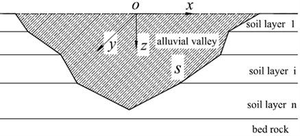
a)
b)
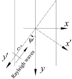
The 3-D responses of the 2-D valley have a unique feature with the wave fields at two different cross sections of the valley being identical but with a shift in phase in the frequency domain. This allows only one cross section of the valley be used for calculation to obtain the whole 3-D dynamic responses, while wave fields at other sections can be obtained by phase offset. In this paper, only the interface of the valley is discretized into inclined straight lines for half-space Green’s functions are used in the proposed IBEM. The total responses are assumed to be the sum of the free-field and scattered-field responses. Firstly, the free-field responses are calculated to determine the displacements and stresses at the interface of the valley, and then one set of fictitious distributed loads and pore pressures moving parallel to the - axis are applied at the line elements (interface of the valley) to represent the scattered wave field outside of the valley (scattered wave field in the layered half-space), and another set of distributed loads and pore pressures on the same line elements to represent the scattered wave field inside of the valley (Fig. 2). The amplitudes of the two sets of fictitious moving distributed loads and pore pressures can be determined by the boundary conditions at the interface of the valley, and finally, the dynamic responses arising from the waves in the free-field and from the fictitious moving distributed loads and pore pressures are summed to obtain the total responses.
Fig. 2Discretization of the interface of the alluvial valley
2.1. Biot’s theory
The equations of motion of a poroelastic medium [13-15] can be expressed as:
where, and are displacement vectors of the solid frame and of the pore fluid with respect to the solid frame, respectively; ; is the displacements vector of the pore fluid; represents the total density; is solid grain’s density; is pore fluid’s density; is porosity; is a parameter that accounts for internal friction due to relative motion between the solid frame and the pore fluid; represents a density-like parameter; is the couple density between the solid grain and the pore fluid; and are Lame’s constants of the solid frame, ; and are Biot’s parameters, which account for compressibility of the two phase material.
To solve the Biot’s governing equations in Cartesian coordinate system, two kinds of Fourier transformation are involved: one with respect to time and frequency, and the other with respect to the two horizontal coordinates and wave numbers. In this paper, the Fourier transformations for the two horizontal coordinates and time are defined as follows:
where , and denote the two horizontal coordinates and time, while , and represent the two horizontal wave numbers and frequency. Performing the Fourier transform on Eq. (1) and solving the resulting ordinary differential equations, the displacement amplitudes of the solid frame and of the pore fluid with respect to the solid frame in the frequency and wave number domain can be written as:
where:
and , , , , , , and are the amplitudes of the up-going and down-going , , and waves, respectively, and , and are the wave numbers associated with the , and waves, which are determined by Eq. (4):
where:
2.2. 3-D stiffness matrix of saturated, layered half-space and solutions of the free field responses
The constitutive equations for a poroelastic medium have the following form [13-15]:
where is the Dirac delta function; represents the dilation of the solid skeleton; represents the volume of fluid injected into a unit volume bulk material; is the stresses in the bulk porous medium; and is the pore pressure.
The displacement amplitudes at the top and the bottom of a saturated layer can be expressed as Eq. (7a) developed based on Eqs. (3), and the external load amplitudes can be expressed as Eq. (7b) based on Eqs. (3) and Eqs. (6), by introducing , , , , , , and =:
where , , , , and are the solid frame’s displacement amplitudes; and are the displacement amplitudes of pore fluid with respect to the solid frame; , , , , and are the total stresses amplitudes; and and are the pore pressure amplitudes. To achieve symmetry, all vertical components in Eq. (7) are multiplied with . Eliminating the amplitudes , , , , , , and in Eq. (7), leads to the 3-D dynamic stiffness matrix of the saturated soil layer . Applying loads at the free surface of the saturated half-space, only down-going waves with amplitudes , , , and are developed, as the radiation condition states that no energy propagates from infinity, it excludes the up-going waves with and . Therefore, by setting 0 in Eq. (8) and eliminating , , and , the saturated half-space matrix can be obtained. Considering the continuity of displacements and equilibrium of stresses and pore pressure at the layer interfaces, the global 3-D stiffness matrix of a multi-layered site are obtained by assembling the layer matrices and the half-space stiffness matrix . Once is obtained, the discretized dynamic-equilibrium equation of the layered saturated site can be expressed as:
where, and are the vector of the displacement amplitudes and vector of external load amplitudes at the interfaces of the saturated layer.
To obtain free-field responses of the incident Rayleigh waves in a layered half-space, the relationship between the apparent velocity and the frequency must be established. Using the 3-D dynamic stiffness matrix of the layered site, the relationship between and can be established by setting . Newton iteration method can be used to obtain the for the given . Substituting these values of in the global dynamic matrix leads to nontrivial solutions for the dynamic-stiffness matrix , which corresponds to the so-called Rayleigh wave modes. Thus, the ratios of displacement amplitudes at the layers’ interfaces are obtained. Once the displacements at the interfaces of the layers are obtained, the amplitudes of the up-going waves and down-going waves in the layers can be determined using Eq. (8a). Then the free-field responses are obtained, which consist of the displacements of the solid frame in the , and directions and the displacement of the pore fluid with respect to the solid phase , and the stresses in the , and directions and pore pressure (Fig. 2). The subscript ‘’ indicates the variables that represent terms in the free-field responses.
2.3. Moving Green’s functions and solutions of the scattered wave field
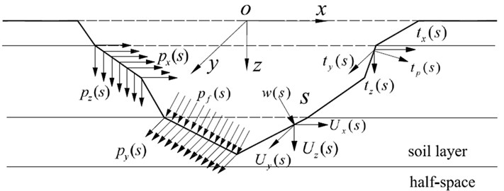
The Green’s functions used in this paper denote the dynamic responses at any point in the free-field system (without the valley) when moving distributed loads in the , and directions and the pore pressures acting on an inclined line embedded in the saturated layered half-space (Fig. 3). These versions of green’s functions for a layered half-space originate from Wolf [22], which were extended to the poroelastic case by Liang et al. [23] and to the 2.5 D form by Ba and Liang [25]. Taking the distributed load in the direction moving along the axis as an example, the load amplitude in the time and space domain, arising from the value of density can be expressed as:
where, (0° 180°) is the angle of the line measured from the horizontal plane and is the moving velocity. can be obtained from Fig. 1(b) for Rayleigh waves with the arriving angle with respect to the axis. is the Rayleigh wave’s velocity of the top soil layer. Performing Fourier transforms with respect to the two horizontal coordinates and also with respect to time on Eq. (9), the load amplitude in the frequency and wave number domain can be expressed as:
Fig. 3Distributed load acting on an inclined line in soil layers
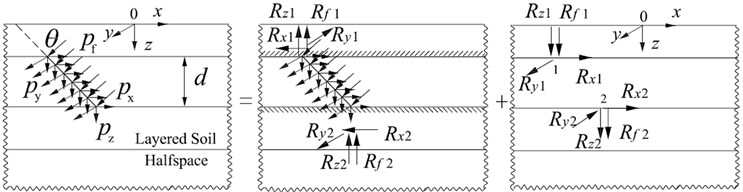
As only part of the layer is loaded, two additional interfaces are introduced at the top and the bottom boundary of the load. First, the layer on which the distributed load acts is fixed at the two interfaces, and the corresponding reaction forces , , , at the top interface and , , , at the bottom interface) are calculated to achieve this condition. This way, the analysis is restricted to the loaded layer. The directions of these forces are then reversed, and are applied as external loads to the total system to determine the global response, and the dynamic responses of the total system induced by the external forces can be implemented using the direct stiffness method. The total response is finally obtained by adding the results of analysis of the fixed layer of the reaction forces (Fig. 3).
It should be noted that the above calculations are performed in the frequency and wave number domain, and the Green’s functions in the time and space domain can be obtained using inverse Fourier transformation given by Eq. (11):
where , is the dynamic response in the frequency and wave number domain, and is the response in the frequency and space domain
Using the Green’s functions described above, the scattered wave fields outside and inside of the valley are simulated by two sets of moving Green’s functions for the layered half space and for the valley, respectively. Therefore, when the free surface is drained (permeable), the displacements and stresses at the interface of the valley arising from the scattered wave fields outside and inside of the valley can be expressed as:
where and are the displacements and stresses Green’s functions for the layered half-space with a drained free surface, and and are the displacements and stresses Green’s functions for the valley. In Eq. (12), the subscript ‘’ indicates results attributable to the moving distributed loads and pore pressures, while the superscripts ‘’ and ‘’ denote parameters associated with the layered half-space and with the valley, respectively. and are the load and pore pressure amplitude vectors acting on the interface to calculate the green’s functions for layered half-space and for the valley, respectively.
Similarly, when the free surface is undrained (impermeable), the displacements and stresses at the interface of the valley arising from the scattered wave fields outside and inside of the valley can be expressed as:
where, , , and are the displacements and stresses Green’s functions for the layered half-space and for the valley with an undrained free surface, respectively.
2.4. Boundary conditions
If the free surface of the layered half-space and the interface of the valley have a drained boundary condition, the boundary conditions at the valley interface can be expressed as:
where, is the weighting function. If takes the value 1 in a single element and zero in all the others, the integral can be evaluated over each element separately. Substituting Eq. (12) into Eq. (14) results in:
where:
Combining the solutions of Eqs. (15) and (12), the displacements and stresses outside of the valley will be:
and the displacements and the stresses inside of the valley will be:
If the free surface of the layered half-space and the interface of the valley are both impermeable (undrained boundary), the boundary conditions are: continuity of the displacements of soil frame, equilibrium of the stresses, and zero flow through the interface of the valley. Similar to the calculation process described above for the drained boundary case, the responses outside and inside of the valley can be obtained for the undrained boundary case.
Fig. 4Surface displacement amplitudes compared with those of Dravinski and Mossessian [7]
![Surface displacement amplitudes compared with those of Dravinski and Mossessian [7]](https://static-01.extrica.com/articles/16148/16148-img5.jpg)
![Surface displacement amplitudes compared with those of Dravinski and Mossessian [7]](https://static-01.extrica.com/articles/16148/16148-img6.jpg)
3. Verification of the method
The present method can be reduced to a 2-D problem in an elastic medium when the incident angle 90° and the saturated parameters , , , and are set as small values (i.e., 10-3). The 2-D results of Rayleigh waves for a semi-circular valley embedded in a uniform elastic half-space provided by Dravinski and Mossessian [7] are used for comparison. The parameters used in the analysis are as follows: Poisson’s ratios of both the valley and the half-space are 1/3, damping ratio is 0.005, the shear wave velocity ratio of the valley to the half-space is 0.5, the mass density ratio is 2/3 (note that the superscript ‘’ represents the valley and ‘’ represents the half-space). The incident frequency 0.5 and 1.0 are defined as , where, is the radius of the valley. Fig. 4 shows that the results from the analysis are in good agreement with those provided by Dravinski and Mossessian [7].
4. Numerical results and discussion
4.1. Responses of a valley in a uniform half-space
A semi-circular saturated valley embedded in a uniform fluid-saturated half-space is first analyzed for both drained and undrained boundary conditions. The material parameters of the half-space and of the valley are presented in Table 1 for the case of 0.3. The internal friction due to relative motion between the solid frame and the pore fluid is not considered in this analysis (i.e. 0). The dimensionless incident frequency is defined as , where and are shear modulus and total density of the saturated half-space, respectively, and is the radius of the valley. Fig. 5 presents the amplitudes of the surface displacement for dimensionless incident frequencies 1.0 and 2.0, incident angles 30°, 60° and 90°. The solid frame displacement amplitudes in the and directions are defined as and , where and are the two free-field horizontal displacements of the obliquely incident Rayleigh waves.
Table 1Parameters for the saturated valley and the saturated half-space
(Pa) | (Pa) | (Pa) | (kg/m3) | (kg/m3) | ||||
Half-space | 0.1 | 156.33E8 | 182.16E8 | 55000 | 2650 | 1000 | 0.25 | 0.2762 |
0.3 | 37E8 | 60.72E8 | 7222 | 2650 | 1000 | 0.25 | 0.8287 | |
Alluvial valley | 0.1 | 39.08E8 | 143.71E8 | 55000 | 2650 | 1000 | 0.25 | 0.2762 |
0.3 | 9.25E8 | 47.92E8 | 7222 | 2605 | 1000 | 0.25 | 0.8287 |
Fig. 5 indicates that the presence of the saturated valley can cause very large amplification of the surface ground motion locally, which is strongly dependent upon the incident angles and the drainage condition. The repeated interference of the transmitted waves in the saturated valley leads to a large amplification on the surface of the valley. The relatively shorter wavelengths in the valley made the amplitude oscillations on the surface more violent. The displacement amplitudes in the left side (i.e., the incident side) of the valley are more complex than those on the right side because of the filtering effect of the valley.
The results in Fig. 5 also show that the 3-D responses (i.e., for 90°) are different from the 2-D case (i.e., for 90°). These results indicate that the obliquely incident wave fields cannot be simply decomposed into in-plane wave fields and anti-plane wave fields, and then be calculated as the total in-plane and anti-plane responses. As the incident angle increased, the displacement amplitudes in the direction increased gradually, while the displacement amplitudes in the direction decreased gradually. For the 2-D case (90°), only the in-plane displacements (displacements in the and directions) are present. The drainage condition also has a significant effect on the surface displacement amplitudes, and the amplitudes are larger and more complex for the undrained boundary condition than those for the drained case. The reason for this phenomenon can be attributed to a stronger ‘encapsulation effect’ in the case of an undrained saturated valley.
Fig. 6 shows the contours of the pore pressure amplitudes in the range of and for 0.5 and 2.0. The incident angles are 30° and 60° and the drainage condition is undrained. The calculation model, material parameters, and also the definition of the dimensionless frequency used are same as for the results presented in Fig. 5. The dimensionless pore pressure amplitudes are defined as .
It can be seen that larger amplitudes and more violent oscillations of pore pressures are found inside the valley compared to those in the outside saturated half-space. The pore pressure amplitudes at the right side of the valley are much larger, in contrary to the distribution of the displacement amplitudes. As the incident frequency increased, the amplitudes of the pore pressure increased significantly and the oscillations became more violent. Fig. 6 also shows that the amplitudes of the pore pressure became larger with increasing incident angle, and increasing incident angle increased the differences in pore pressure amplitudes between the left and right side of the valley.
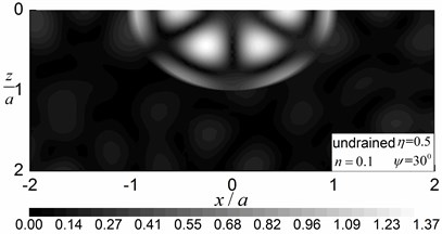
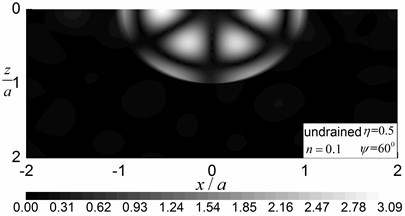
Fig. 7 shows the contours of the amplitudes of the pore pressure in the range of and for 0.5, with an undrained boundary condition and 30°and 60°. The material parameters of the saturated half-space and of the saturated valley are presented in Table 1 for the case of 0.1 and the internal friction is not considered (0). Comparisons between the results in Fig. 7 (0.3) and results in Fig. 6 (0.1) show that porosity has significant effect on wave scattering around the valley. As the porosity decreased, the pore pressure amplitudes decreased significantly, while the oscillations of the pore pressures became more violent. This indicates that less energy is taken up by the pore fluid than by the solid frame. The results in Fig. 7 also show that the pore pressure amplitudes become more concentrated inside the valley for smaller porosity (i.e. 0.1).
Fig. 5Surface displacements amplitudes for different obliquely incident angels (n= 0.3)
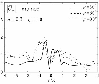
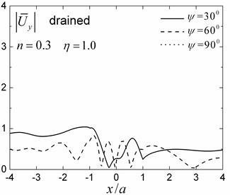
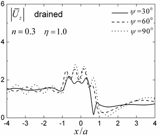
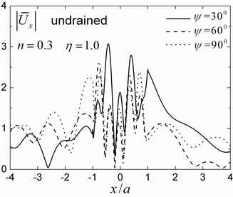
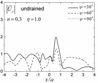
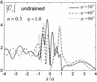
Fig. 6Contours of pore pressure amplitudes around the valley (n= 0.3)
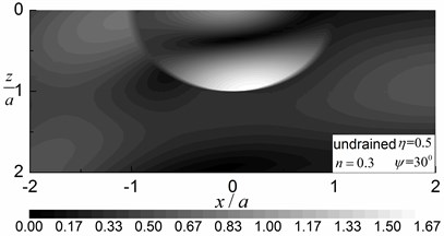
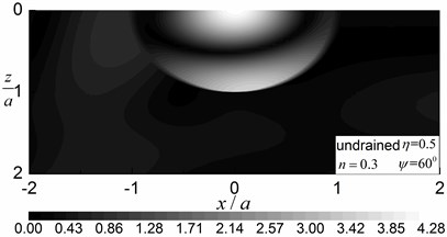
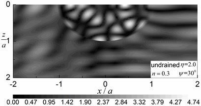
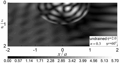
Fig. 7Contours of pore pressure amplitudes around the valley (n= 0.1)
4.2. Responses of a valley in a layered half-space
A semi-circular valley embedded in a single elastic layer overlying an elastic half-space is analyzed considering both drained and undrained boundary conditions. The material parameters of the saturated valley are shown in Table 1 for the case of 0.3 and material damping ratio of 5 % is considered in this analysis. The material parameters of the elastic layer are as follows: mass density 1855 KN/m3, shear modulus 3.7 MPa, Poisson’s ratio 0.25 and damping ratio 5 %. The material parameters of the underlying elastic half-space are as follows: 1855 KN/m3, shear modulus ratio of the half-space to the layer is 5.0, Poisson’s ratio 0.25 and damping ratio 2 %. The thickness of the layer is 2.0 and the incident angle is 45°. The dimensionless incident frequency is defined as . Fig. 8 shows the amplitudes of the surface displacement for the first three modes of the Rayleigh waves for 1.0 and 2.0. The displacement amplitudes in the , and directions are defined as and , where and are the two free-field horizontal displacements of the obliquely incident Rayleigh waves in the layered half-space.
Results presented in Fig. 8 indicate that the surface displacement amplitudes can vary with different Rayleigh modes, depending on the dimensionless frequency and drainage conditions. Largest vertical displacement amplitudes are found in the third Rayleigh mode with maximum vertical displacement amplitudes at 2.2, 2.4 and 9.4, for Rayleigh modes 1, 2 and 3, respectively, for 1.0. The largest vertical displacement amplitudes occurred at the second mode for 2.0 with the maximum vertical displacement amplitudes at 2.2, 4.1 and 1.2 for the Rayleigh mode 1, 2 and 3, respectively, for 2.0).
Fig. 8Surface displacement amplitudes for the first three modes (GR/GL= 5, H/a= 2.0)
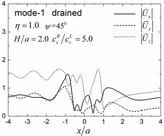
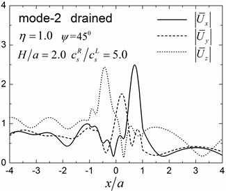
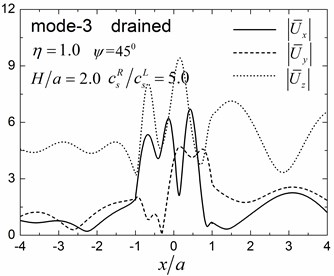
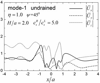
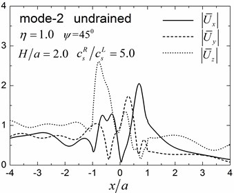
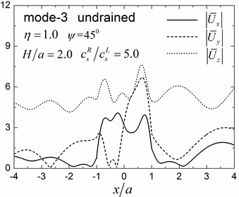
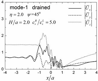
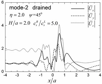
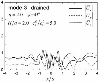
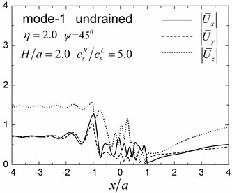
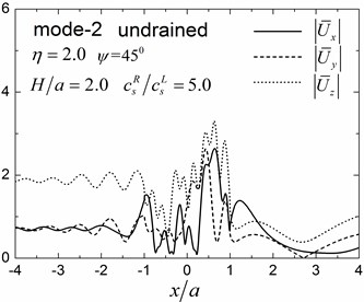
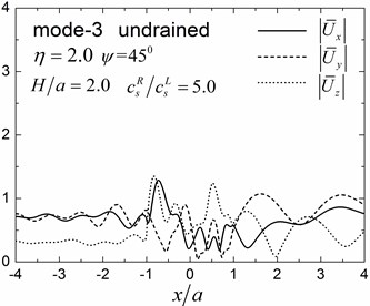
Fig. 9 shows pore pressure amplitude contours inside of the valley for the first three Rayleigh modes, with dimensionless frequency 1.0 and 2.0, and incident angle 45°. Both the drained and undrained boundary conditions are considered in the analysis. The calculation model and material parameters are same as those in Fig. 8. The pore pressure amplitudes in Fig. 9 are defined as .
Fig. 9 shows that both the values and the spatial distributions of the pore pressure amplitudes are different for different Rayleigh modes, depending on the incident frequency, incident angle, and the drainage condition. The pore pressure amplitude is largest at the third Rayleigh mode for 1.0, while it is largest at the second Rayleigh mode for 2.0. The oscillations of the pore pressure amplitudes are most violent for the first Rayleigh mode, less violent for the second Rayleigh mode, and the least violent for the third Rayleigh mode, which may be attributed to the faster apparent velocity (corresponding to longer wavelength) for the higher Rayleigh modes (Table 2). With increasing incident frequency, the pore pressure amplitudes become larger and the spatial distributions become more complex. It can also be seen for Fig. 9 that the drainage boundary condition has significant effects on the values and spatial distributions of the pore pressure amplitudes and the oscillations are more violent for the undrained boundary condition.
Fig. 10 shows the amplitudes of the surface displacement and Fig. 11 shows the contours of pore pressure amplitudes inside of the valley for the first two Rayleigh modes, illustrating the effects of the stiffness of the soil layer. In this results, the same calculation model and the same materials as in Fig. 9 are used, except the shear modulus ratio of the half-space to the layer is 2.0.
By comparing the results in Fig. 8 and Fig. 9 with Fig. 10 and Fig. 11 for 1.0, it can be seen that the values and the spatial distributions of displacement (pore pressure) amplitudes are similar for the first Rayleigh mode, but are significantly different for the second mode. This is because for the scattered Rayleigh waves in a layered site, the resulting responses depend on two aspects: (1) the dynamic interaction between the valley and the layered site, and (2) the dispersion characteristics of the Rayleigh waves. The large difference in the apparent velocity of the second mode (Table 2) leads to the significant difference in the dynamic responses in Figs. 8-9 and in Figs. 10-11, although the dynamic interaction keep invariant for the unchanged thickness of the layer (The dynamic interaction is determined by the thickness of the layer for invariant shape of valley).
Fig. 9Contours of pore pressure amplitudes for the first three modes (GR/GL= 5, H/a= 2.0)
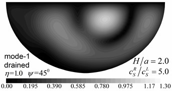
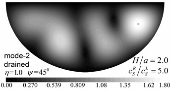
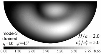
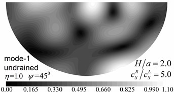
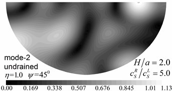
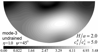
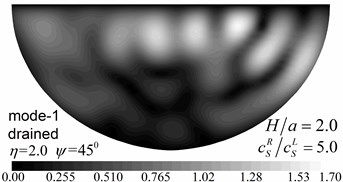
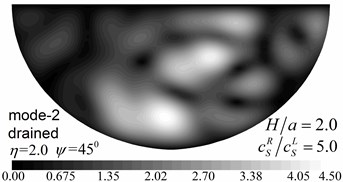
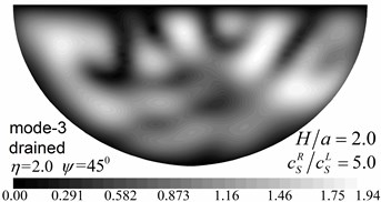
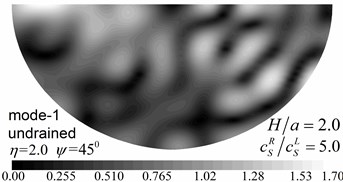
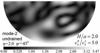
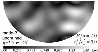
Fig. 10Surface displacement amplitudes for the first two modes (GR/GL= 52, H/a= 2.0)
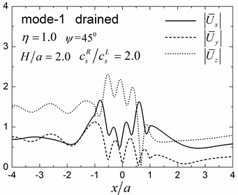
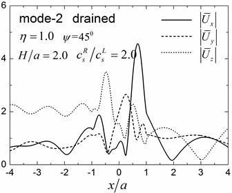
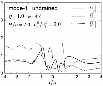
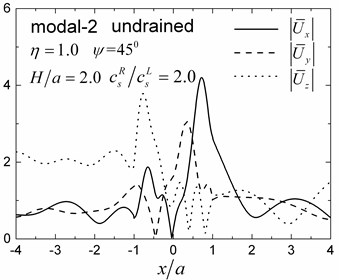
Fig. 11Contours of pore pressure amplitudes for the first two modes (GR/GL= 2, H/a= 2.0)
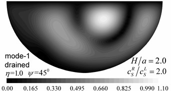
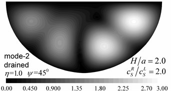
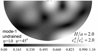
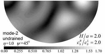
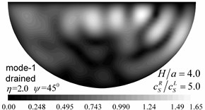
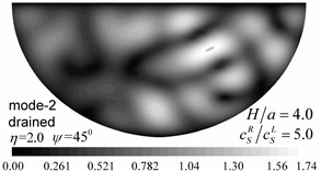
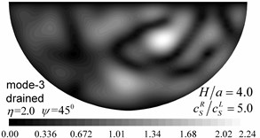
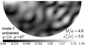
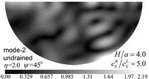
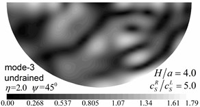
Fig. 12 shows the amplitudes of the surface displacement and Fig. 13 shows the contours of pore pressure amplitudes inside of the valley for the first three Rayleigh modes, illustrating the effects of the soil layer thickness. The same materials and calculation model are used as in Fig. 9, except that the thickness of the layer is 4.0.
By comparing the results in Fig. 12 and Fig. 13 with results in Fig. 8 and Fig. 9 for 2.0, it can be seen that the values and spatial distributions of the displacement (pore pressure) amplitudes are different for all three modes, which may be attributed to the changed dynamic interaction between valley and layered site (due to changes in the thickness of the layer) and also to the different values of the apparent velocity for the two layered half-space (Table 2). It can also be seen from Fig. 12 and Fig. 13 that the values and spatial distributions of the displacement (pore pressure) amplitudes are very similar for the second and the third modes because of the closer apparent velocities of the two modes (Table 2).
Fig. 12Surface displacement amplitudes for the first three modes (GR/GL= 5, H/a= 4.0)
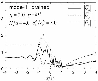
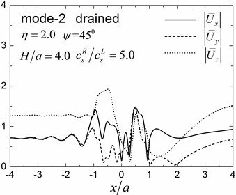
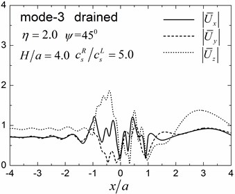
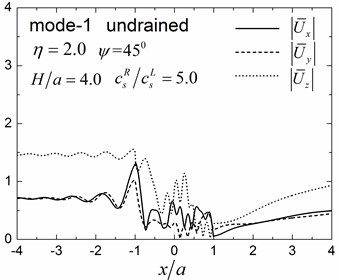
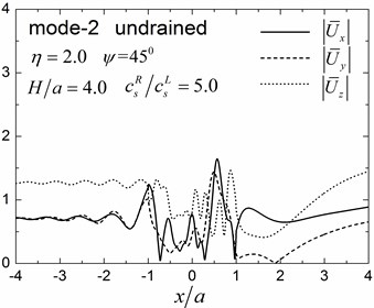
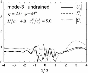
Table 2Apparent velocities for the first three Rayleigh modes
5, 2 | 2, 2 | 5, 4 | ||
1.0 | 2.0 | 1.0 | 2.0 | |
Mode-1 | 1309.88+67.76 | 1301.69+64.94 | 1308.56+67.17 | 1301.69+64.94 |
Mode-2 | 2226.44+156.01 | 1511.82+89.30 | 2085.67+133.77 | 1431.49+73.30 |
Mode-3 | 3524.38+388.14 | 2413.09+149.86 | 1517.60+99.14 | |
For layered half-space of 2 and 2, there are no higher modes than the second mode at the frequency 1.0 | ||||
Fig. 13Contours of pore pressure amplitudes for the first three modes (GR/GL= 5, H/a= 4.0)
5. Conclusions
The 3-D scattering of obliquely incident Rayleigh waves by a saturated alluvial valley embedded in a layered half-space is studied using the indirect element method in the frequency domain. Results from the analysis indicated that as the porosity decreased, the pore pressure amplitude values decreased significantly, while the oscillations became violent. The values and spatial distributions of the displacements amplitudes and of the pore pressure varied with the Rayleigh modes. The higher Rayleigh modes resulted in longer wavelengths and lead to simpler spatial distributions. The responses around the valley are determined by the dynamic interaction between valley and layered half-space, and the dispersion characteristics of the Rayleigh waves for a given layered half-space.
References
-
Aki K., Larner K. L. Surface motion of a layered medium having an irregular interface due to incident plane SH waves. Journal of Geophysical Research, Vol. 75, 1970, p. 1921-1941.
-
Trifunac M. D. Surface motion of a semi-cylindrical alluvial valley for incident plane SH waves. Bulletin of the Seismological Society of America, Vol. 61, 1971, p. 1755-1770.
-
Wong H. L., Trifunac M. D. Surface motion of a semi-elliptical alluvial valley for incident plane SH waves. Bulletin of the Seismological Society of America, Vol. 64, 1974, p. 1389-1408.
-
Yuan X., Liao Z. Scattering of plane SH waves by a cylindrical alluvial valley of circular-arc cross-section. Earthquake Engineering and Structural Dynamics Journal, Vol. 24, 1995, p. 1303-1313.
-
Todorovska M., Lee V. W. Surface motion of shallow circular alluvial valleys for incident plane SH waves: analytical solution. Soil Dynamics and Earthquake Engineering, Vol. 4, 1991, p. 192-200.
-
Dravinski M. Scattering of plane harmonic SH wave by dipping layers or arbitrary shape. Bulletin of the Seismological Society of America, Vol. 73, 1983, p. 1303-1319.
-
Dravinski M., Mossessian T. K. Scattering of plane harmonic P, SV, and Rayleigh waves by dipping layers of arbitrary shape. Bulletin of the Seismological Society of America, Vol. 77, 1987, p. 212-235.
-
Liang Ba J. W. Z. N. Surface motion of an alluvial valley in layered haft-space for incident plane SH waves. Earthquake Engineering and Engineering Vibration, Vol. 27, 2007, p. 1-9, (in Chinese).
-
Sainchez-Sesma F. J., Ramos-Martinez J., Campillo M. An indirect boundary element method applied to simulate the seismic response of alluvial valleys for incident P, S and Rayleigh Waves. Earthquake Engineering and Structural Dynamics Journal, Vol. 22, 1993, p. 279-295.
-
Kawase H., Aki K. A study on the response of a soft basin for incident S,P and Rayleigh waves with special reference to the long duration observed in Mexico City. Bulletin of the Seismological Society of America, Vol. 79, 1989, p. 1361-1382.
-
Boore D. M., Larner K. L., Aki K. Comparison of two independent methods for the solution of wave scattering problems: response of a sedimentary basin to incident SH waves. Journal of Geophysical Research, Vol. 76, 1971, p. 558-569.
-
Bouchon M. Effect of topography on surface motion. Bulletin of the Seismological Society of America, Vol. 63, 1973, p. 615-632.
-
Biot M. A. The theory of propagation of elastic waves in a fluid-saturated porous solid I: low-frequency range. The Journal of the Acoustical Society of America, Vol. 28, 1956, p. 168-178.
-
Biot M. A. The theory of propagation of elastic waves in a fluid-saturated porous solid II: Higher-frequency range. The Journal of the Acoustical Society of America, Vol. 28, 1956, p. 179-191.
-
Biot M. A. Mechanics of deformation and acoustic propagation in porous media. Journal of Applied Physics, Vol. 33, 1962, p. 1482-1498.
-
Zhou X., Jiang L., Wang J. Scattering of plane wave by circular-arc alluvial valley in a poroelastic half-space. Journal of Sound and Vibration, Vol. 318, 2008, p. 1024-1049.
-
Liu Z., Liang J. Diffraction of plane P waves around an alluvial valley in poroelastic half-space. Earthquake Science, Vol. 23, 2010, p. 35-43.
-
Li W., Zhao C. Scattering of plane SV waves by circular-arc alluvial valleys with saturated soil deposits. Soil Dynamics and Earthquake Engineering, Vol. 25, 2005, p. 981-995.
-
Pedersen H., Sanchez Sesma F.-J., Campillo M. Three-dimensional scattering by two-dimensional topographies. Bulletin of the Seismological Society of America, Vol. 84, 1994, p. 1169-1183.
-
De Barros F. C. P., Luco J. E. Amplication of obliquely incident waves by a cylindrical valley embedded in a layered half-space. Soil Dynamics and Earthquake Engineering, Vol. 14, 1995, p. 163-175.
-
Liang J., Wei X., Lee V. W. 3D scattering of plane SV waves by a circular-arc alluvial valley. Chinese Journal of Geotechnical Engineering, Vol. 31, 2009, p. 1345-1353, (in Chinese).
-
Wolf J. P. Dynamic Soil-Structure Interaction. Englewood Cliffs, Prentice-Hall, NJ, 1985.
-
Liang J., You H. Green’s functions for uniformly inclined line distributed loads acting on an inclined line in a poroelastic layered site. Earthquake Engineering and Engineering Vibration, Vol. 4, 2005, p. 233-241.
-
Liang J., You H., Lee W. W. Scattering of SV waves by a canyon in a fluid-saturated, poroelastic layered half-space, modeled using the indirect boundary element method. Soil Dynamics and Earthquake Engineering, Vol. 26, 2006, p. 611-625.
-
Ba Z., Liang J. 2.5D Scattering of incident plane SV waves by a canyon in layered half-space. Earthquake Engineering and Engineering Vibration, Vol. 9, 2010, p. 587-595.
About this article

This study is supported by National Natural Science Foundation of China under Grant No. 51578373 and 51578372, and Tianjin Research Program of Application Foundation and Advanced Technology under Grant No. 12JCQNJC04700, which is gratefully acknowledged.
