Abstract
By combining the wave function expansion method with the auxiliary function, a closed series solution for the dynamic plane response is proposed considering horizontal circular heterogeneous topography under SH wave incidence. The displacement and stress residual is found to be small along the entire boundary, including the corner points; further, the solution can be used for the incidence of a high-frequency wave. In this study, the influence of the shear modulus ratio of a heterogeneous hill and a lower medium on the displacement amplitude spectrum and surface displacement is determined. The results show that the hardness of the medium in hill topography significantly influences out-of-plane surface motion. The surface displacement of the soft hill is significantly larger than that of the homogeneous hill, and the motion effects are enhanced considerably. In contrast, the hard hill weakens surface motion.
Highlights
- The number of series iteration is more with the increase of frequency of incident wave to ensure the calculation accuracy.
- The incident angle, dimensionless frequency, and shear modulus ratio of the heterogeneous hill and lower medium have a great influence on surface displacement.
- Because of the high calculation accuracy, it is possible to study the characteristics of surface.
1. Introduction
The site response problem is an important wave problem in seismic engineering. Several seismic damage data show that local terrains have a great impact on the scattering and diffraction of seismic waves. In recent years, large-scale infrastructure development has been carried out in many cities globally, where raised terrains are common in engineering sites. Engineering structures near mountainous areas should consider the amplification effect of the terrain. Therefore, exploring the scattering law of seismic waves by heterogeneous protrusion has high theoretical significance and clear engineering reference value.
Various field measurements have shown that variations in topographic configuration influence the intensity of ground motion [1-5]. Numerous mathematical models provide insight into the behavior of ground shaking due to geologic and topographic variations. Most closed-form analytical solutions are related to the irregularities of subsurface, such as horizontally stratified surface layers [6], semi-circular canyons or valleys [7, 8], semi-elliptical canyons or valleys [9, 10], and circular underground cavities or tunnels [11, 12].
However, for the surface convex or hill topography, the scattering of elastic waves in hills is also a challenging problem due to mixed boundary value. According to earthquake investigators, the amplification effect of actual hill topography is much larger than the theoretical results. Some scholars speculate that it is caused by the difference in properties between hill topography and the underlying medium [13]. Based on the method of partition and auxiliary function, Yuan et al. [14-16] proposed the auxiliary function and the external region Graf addition formula and obtained the closed-level solution for the SH-wave scattering by semi-circular and arbitrary circular hill topography. Based on the above theory, Vincent [17, 18] used an improved wave function expansion method to resolve the analytical solution of the SH wave scattering of the semi-circular convex terrain. Li and Yuan [19] used the auxiliary function method and wave function expansion to obtain an out-of-plane dynamic response of heterogeneous protrusions in half-space. Tsaur et al. [20] solved the scattering of plane SH waves by arc-arc-convex terrain and obtained the corresponding series solution. Tsaur [21] also studied the scattering of SH wave by semi-elliptical convex terrain and calculated the steady-state response. Amornwongpaibun et al. [22] proposed an analytical solution for the closed-wave function of two-dimensional scattering and diffraction of SH waves in a semi-elliptical shallow hill with a concentric elliptical tunnel in a semi-elastic half-space. Liu et al. [23] investigated the dynamic interaction between a lined tunnel and a hill under plane SV waves using the indirect boundary element method.
In this study, an improved wave function method is used to solve the out-of-plane dynamic response of a half-space heterogeneous hill. The wave function is expanded into a cosine function by Fourier series [11]. The solution is reduced to a set of infinite algebraic equations; a numerical solution can then be obtained from the truncation of the infinite equations. The calculation results show that the displacement and stress residual is minimal and can be ignored along the entire boundary, including the corner points. The calculation accuracy is quite high and the method can offer effective solutions for high-frequency waves. Based on the improved wave function method, the effect of key factors, such as the angle and frequency of the incident wave and material property of hill on the dynamic response, is investigated, and the conclusions will help with the seismic design of underground mountain structures.
2. Physical model
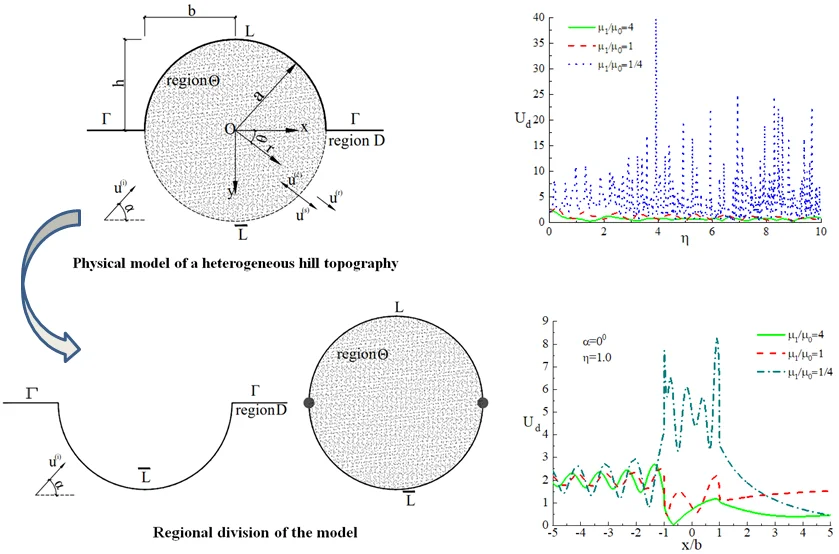
The cross-section of the model is shown in Fig. 1. It is identical to that considered by Yuan and Men [14]. It represents a homogeneous, isotropic, and fully elastic half-space with a semi-circular hill of radius . and denote the shear modulus and wave velocity of the half-space, respectively. and denote the shear modulus and wave velocity of the circular hill, respectively. The flat surface boundary is recorded as , and the height and half-width of the hill topography are and , respectively. This can be written as .
Fig. 1Physical model of a heterogeneous hill topography
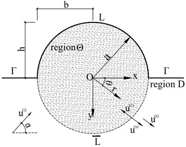
Fig. 2Regional division of the model
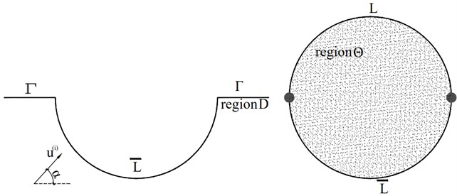
As shown in Fig. 2, the physical model is divided into two regions. Region is the circular region including the circular hill, in which the upper and lower boundaries are denoted as and , respectively. Region forms the rest of the half-space. The common boundary of regions and is , and the flat surface beyond the hill is denoted by . By dividing the original complex model into two completely independent small circular or flat boundary regions, the wave fields in these regions can be represented by the Fourier-Bessel wave function. When combined with the continuity of displacement and stress between the two regions, the boundary conditions of the original model can be derived. The remaining boundary conditions for the waves are as follows:
(1) Stress-free conditions at hill boundary in region .
(2) Stress-free conditions at flat surface in the region .
(3) Continuity of displacement and stress at .
3. Numerical model
3.1. Scattered waves: wave function series expansion
Assuming that the displacement of SH wave donated by is excited on the half-space medium, it can be represented in Cartesian coordinate system by:
where , and are phase velocity of the incident wave in the and directions, respectively, , , , and denote the velocity, circular frequency, incidence angle, and amplitude of the incident SH wave.
When the incident wave goes through the hill, the total displacement field should satisfy the wave differential equation [24]:
The stress field should appropriate the stress-free boundary conditions, which is given by:
where:
where, is the shear modulus of the medium of half space soil.
The displacement field of the concave half-space can be expressed as:
where denotes the displacement of free field excited by incident SH wave, denotes the scattering potential field due to the interaction between the fictitious hill boundary and half space.
The free field displacement consists of the incident wave displacement and the reflected wave displacement , which is excited by at the flat surface of half-space:
The equation of incident wave is as shown in Eq. (1). The equation of reflected wave can be represented as:
In Eq. (1) and Eq. (9), is the harmonic factor and can be omitted in subsequent wave expressions. denotes the wave number. Substituting both and into Eq. (1) and Eq. (9) gives:
According to the coordinate transformation relationship , . Eq. (10) will be thus be changed to Eq. (11):
Substituting Eq. (11) into Eq. (8) gives:
where is Bessel function of the first kind with order n, , are the coefficients of free-field waves, , for 1, 2, 3….
Substituting Eq. (12) into Eq. (6):
where , is amplitude of the incident wave stress. It is derived from the expansion theorem of Bessel functions [1] and used extensively [11, 25-29].
Solving the total wave Eq. (2) according to the separation variable method, the expression of the scattering displacement field generated by the semicircular boundary satisfy Eq. (2) and the boundary condition Eq. (3). It can be taken as:
where is an unknown coefficient of the new waves to be determined. is a Hankel function of the first kind with the order .
Substituting Eq. (14) into Eq. (5):
The equation of the stress-free boundary condition Eq. (3) is always automatically satisfied on the boundary (). By substituting Eq. (15) into Eq. (6), we get:
The displacement field of the cohesive wave generated in region owing to the fictitious boundary and the arc-shaped hill surface can be expressed as:
where and are unknown coefficients of new waves to be determined.
The Fourier-Bessel series expansions of all incident waves and scattered waves in each coordinate system are thus obtained.
3.2. A new analytical method after half range expansion of cosine function
To divide the boundary into two parts processed separately, the wave function must be expanded into an orthogonal trigonometric form in the upper and lower semi-regions. The sine and the cosine functions are found to be orthogonal over the entire range but not between the upper and lower ranges. In this case, problems can be solved by using the orthogonal cosine function in the upper and lower half ranges. This method has solved the analytical solution of the scattering of SH waves by semi-circular hill topography [10].
3.2.1. Referencing half range expansion of cosine function
The cosine function is orthogonal in the half range and . Any function can be expanded by using the cosine series function in the range as:
where:
Using Eq. (19), the sine function can be expressed at half ranges of and as:
where, 1, 2, 0, 1, 2, 3,….
3.2.2. Reformulation of the relevant displacement field
The cohesive waves generated in the circular region owing to the fictitious boundary and the arc-shaped hill surface are represented as orthogonal cosine functions in the half ranges and :
Substituting Eq. (21), Eq. (6) takes the form:
3.3. Transformation of boundary conditions
The Fourier-Bessel expressions of various scattered waves in all regions are obtained. The boundary conditions are introduced to establish a system of equations for each group of undetermined coefficients.
(1) the continuity condition of displacement and stress at the boundary .
(2) stress-free boundary condition on circular hill surfaces:
Substituting the corresponding wave function into Eqs. (23-25), we obtain:
3.4. Referencing equation elimination to determine the unknown coefficients
Eqs. (26-28) contain three series of equations for solving three sets of unknowns , , and . There are a variety of methods to solve the unknowns, and one of them is listed below.
From Eqs. (27-28), we obtain:
Deformation of Eq. (29):
Substituting Eq. (29) into Eq. (26):
From Eq. (28) and Eq. (30), the following equations can be obtained:
The solution is obtained by solving a set of infinite algebraic equations. The unknown coefficients are determined by equation truncation. The unknowns , ,and can be obtained from Eqs. (31), (28), and (29), respectively.
4. Numerical analysis
It is necessary to check convergence by calculating the displacement and stress residuals on every boundary. The residuals include:
(1) The continuity of displacement and stress at between region and region .
(2) The stress-free conditions at the hill boundary have the dimensionless displacement residual and the residual stress on the common boundary , respectively.
(3) Stress residual at the hill boundary :
The stress residual of the free surface is strictly satisfied when the wave function is set and will not be discussed here.
The nature of the SH wave is determined by frequency and wave velocity. Wave velocity depends on the physical properties of half-space, from which the wavelength can be determined. At the same time, the influence of waves on surface displacement has a great relationship with the geometrical characteristics of topography and the wavelength. To consider this influence, the dimensionless frequency is introduced and defined as the ratio of the hill diameter 2 to the wavelength of the incident wave .
The formula is:
The characteristic length of topography takes the half-width of hill topography. The numerical results depend on the dimensionless frequency , shear modulus ratio of the heterogeneous hill to adjacent medium and incidence angle of the wave .
The data analysis is divided into four sections from 4.1-4.4. They are convergence and accuracy analysis; a set of typical examples; the influence of shear modulus ratio of heterogeneous hill and lower medium on surface displacement; and the influence of shear modulus ratio of heterogeneous hill and lower medium on displacement amplitude spectrum.
4.1. Convergence and accuracy analysis
Fig. 3 shows the variation of residual of hill surface displacement with the iteration number at the dimensionless frequencies 1.0, 3.0, 5.0, 10.0, for 1/4, 90°, in which NUM is the iteration number of the series for each calculation, e is the root mean square of the iterative residuals. NUM reaches enough small value when it equals to 20, 35, 40, and 60, respectively. It can be seen that the number of series iteration is more with the increase of frequency of incident wave to ensure the calculation accuracy.
Fig. 3Series convergence analysis graph
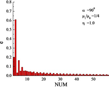
a) Iterative displacement residual graph on surface of hill when 1.0
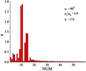
b) Iterative displacement residual graph on surface of hill when 3.0
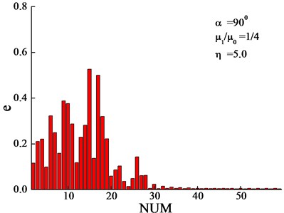
c) Iterative displacement residual graph on surface of the hill when 5.0
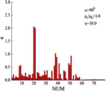
d) Iterative displacement residual graph on surface of the hill when 10.0
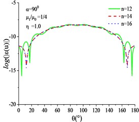
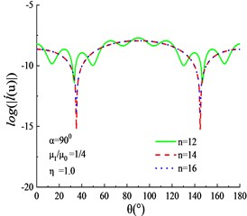
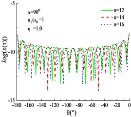
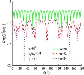
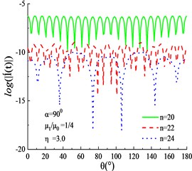
Figs. 4-7 show the displacement and stress residual amplitudes at the boundaries under four different dimensionless frequencies when 1/4. It can be seen that the residual on the entire boundary is so small that it is negligible.
Fig. 4Displacement and stress residual amplitude on various boundaries for μ1/μ0= 1/4, η= 1.0, α= 90°: a) displacement residual amplitude on L, b) stress residual amplitude on L¯, c) stress residual amplitude on L
a)
b)
c)
Fig. 5Displacement and stress residual amplitude on various boundaries μ1/μ0= 1/4, η= 3.0, α= 90°: a) displacement residual amplitude on L, b) stress residual amplitude on L¯, c) stress residual amplitude on L
a)
b)
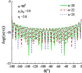
c)
4.2. Typical examples
The amplitude of dimensionless displacement on the free surface is defined as:
where and are the real and imaginary part of surface displacement , respectively.
Fig. 6Displacement and stress residual amplitude on various boundaries μ1/μ0= 1/4, η= 5.0, α= 90°: a) displacement residual amplitude on L, b) stress residual amplitude on L¯, c) stress residual amplitude on L
a)
b)
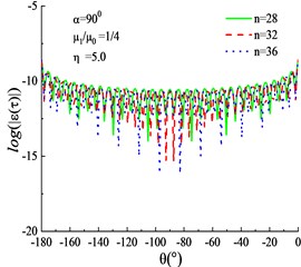
c)
Fig. 7Displacement and stress residual amplitude on various boundaries for μ1/μ0= 1/4, η= 10.0, α= 90°: a) displacement residual amplitude on L, b) stress residual amplitude on L¯, c) stress residual amplitude on L
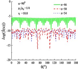
a)
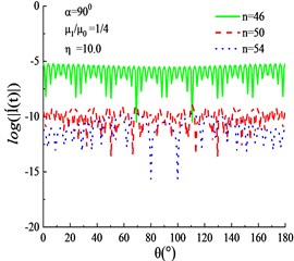
b)
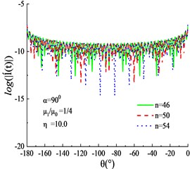
c)
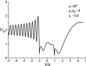
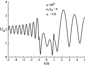
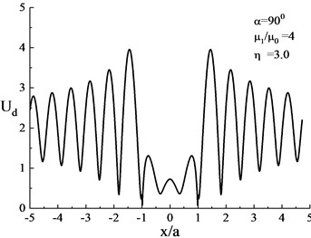
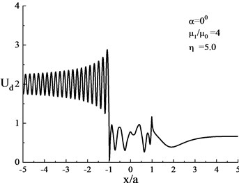
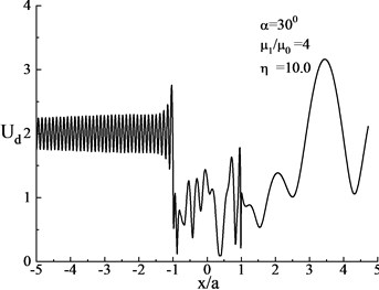
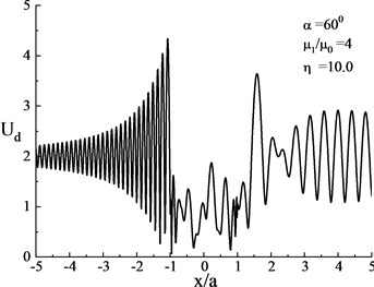
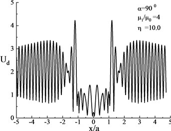
For convenience to compare the results of various numerical and analytical methods with the results given in this paper. Figs. 8-15 show eight typical examples. It shows that the incident angle, dimensionless frequency, and shear modulus ratio of the heterogeneous hill and lower medium have a great influence on surface displacement.
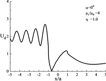
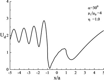
The calculation parameters include (1) shear modulus ratio of heterogeneous hill and lower medium 1/4, 4); (2) dimensionless frequency: 1.0, 3.0, 5.0, 10.0 (3) four angles of incidence: 0°, 30°, 60°, 90°. In this section, the abscissa of the surface displacement map is defined as , where a is the radius of the semi-circular hill.
It can be seen from Figs. 8-15 that as the frequency of incident wave increases, the surface displacement changes more severely, especially for the hill topography. When the incidence angle becomes small, the surface displacement on the left side of hill is more severe than that on the right side, which explains the protection effect of hill topography being similar with the actual vibration isolation trench. In addition, for the case of normal incidence of seismic waves, especially when the wavelength of the incident wave is close to the dimension of hill topography, the surface displacement is minimal near the corner of the hill, which is consistent with actual earthquake damage.
Fig. 8Surface displacement amplitude when the shear modulus ratio of the heterogeneous hill and the lower medium is (μ1/μ0= 1/4, η= 1.0)
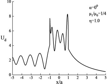
a)0°
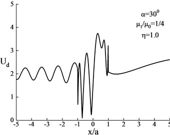
b)30°
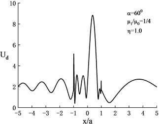
c)60°
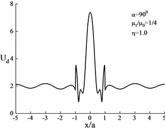
d)90°
Fig. 9Surface displacement amplitude when the shear modulus ratio of the heterogeneous hill and the lower medium is (μ1/μ0= 1/4, η= 3.0)
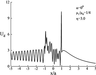
a)0°
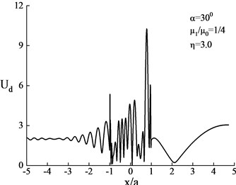
b)30°
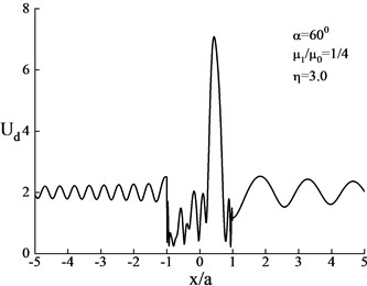
c)60°
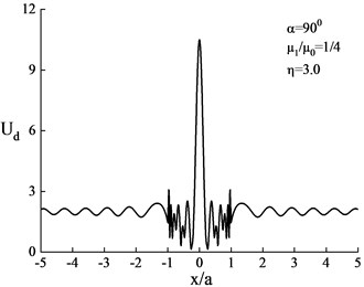
d)90°
Fig. 10Surface displacement amplitude when the shear modulus ratio of the heterogeneous hill and the lower medium is (μ1/μ0= 1/4, η= 5.0)
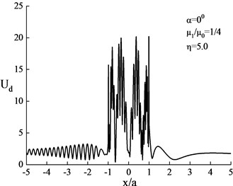
a)0°
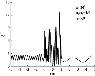
b)30°
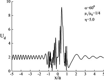
c)60°
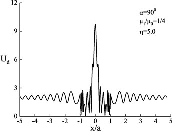
d)90°
Fig. 11Surface displacement amplitude when the shear modulus ratio of the heterogeneous hill and the lower medium is (μ1/μ0= 1/4, η= 10.0)
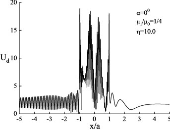
a)0°
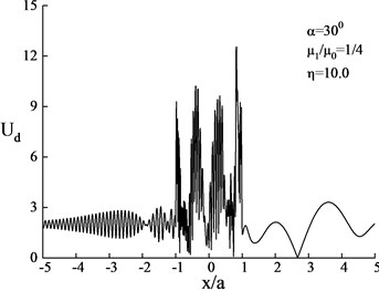
b)30°
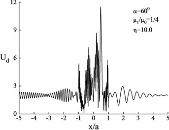
c)60°
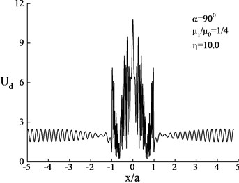
d)90°
Fig. 12Surface displacement amplitude when the shear modulus ratio of the heterogeneous hill and the lower medium is (μ1/μ0= 4, η= 1.0)
a)0°
b)30°
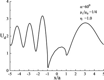
c)60°
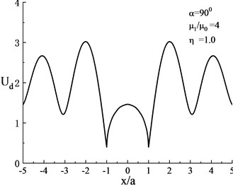
d)90°
Fig. 13Surface displacement amplitude when the shear modulus ratio of the heterogeneous hill and the lower medium is (μ1/μ0= 4, η= 3.0)
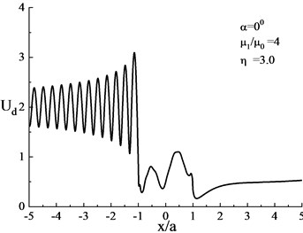
a)0°
b)30°
c)60°
d)90°
Fig. 14Surface displacement amplitude when the shear modulus ratio of the heterogeneous hill and the lower medium is (μ1/μ0= 4, η= 5.0)
a)0°
b)30°
c)60°
d)90°
Fig. 15Surface displacement amplitude when the shear modulus ratio of the heterogeneous hill and the lower medium is (μ1/μ0= 4, η= 10.0)
a)0°
b)30°
c)60°
d)90°
4.3. The influence of the shear modulus ratio of the heterogeneous hill to adjacent medium on surface displacement
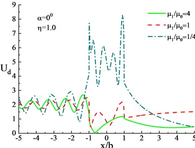
According to the results from Sections 4.1 and 4.2, the shear modulus ratio of the heterogeneous hill and the lower medium has a significant effect on the surface displacement. Therefore, it is necessary to compare the shear modulus ratios of the heterogeneous hill with the lower medium at different time ranges. In this section, the abscissa of the surface displacement map is defined as , where is the half width of the hill topography.
The calculation parameters then include (1) shear modulus ratio of heterogeneous hill and lower medium on semi-circular hill (10), 1/4, 1, 4; (2) dimensionless frequency 1.0, 3.0, 5.0, 10.0; (3) two angles of incidence 0°, 90°.
Fig. 16Surface displacement under influence of different shear modulus ratios of heterogeneous hill and the lower medium (η= 1.0)
a)0°
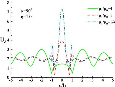
b)90°
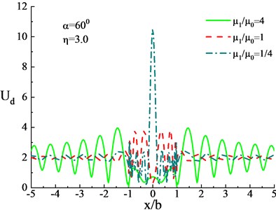
Fig. 17Surface displacement under influence of different shear modulus ratios of heterogeneous hill and the lower medium (η= 3.0)
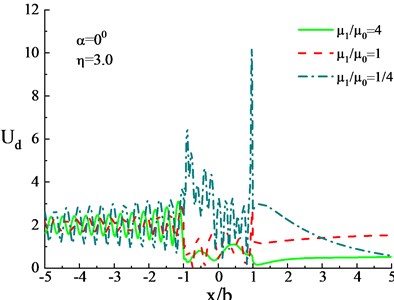
a)0°

b)90°
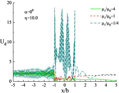
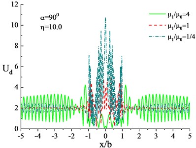
Figs. 16-19 show the amplitude of surface displacement near the hill in cases with the hill topography under three different hardness (1/4, 1, 4)) with the different frequency ( 1.0, 3.0, 5.0, 10.0). In these figures, (a) and (b) indicate the effects of two different angles ( 0°, 90°) of incident waves
It can be noted that the displacement amplitude of the free surface is constant at 2. Figs. 16-19 indicate that the medium hardness of hill topography has a great influence on the surface amplification. Regardless of the incidence angle of the wave, compared with the homogeneous hill, the surface displacement of the soft hill increases significantly, and that of hard hill reduces. This difference between surface displacement is quite large, for vertical incidence of wave, when the medium hardness of hill changes from hard () to soft ( 1/4). For 1.0 the maximum amplitude of hill top changes from 1 (0.5 times surface displacement of free field without hill) to 8 (4 times surface displacement of free field without hill); the maximum amplitude of hill top changes from 0.5 to 10 for 3.0 and from 0.25 to 11 for 10.0.
In addition, the location of the maximum displacement of the hill surface is mainly affected by the incidence angle of waves. The surface displacement on the hill midpoint is prone to amplification for the vertical incidence of the wave. For the grazing incidence of the wave, the amplification of hill surface displacements appears on the back top of the hill, and the location of the maximum displacement of hill surface will move toward the right hill surface with an increase in incidence angle. The motion of the horizontal surface at the hill back will reduce due to the protective effect of the hill, the surface motion fluctuation effect will enhance with increasing frequency of incident wave, and the displacement amplitude of the hill surface will change very sharply for the high-frequency wave.
Fig. 18Surface displacement under influence of different shear modulus ratios of heterogeneous hill and the lower medium (η= 5.0)
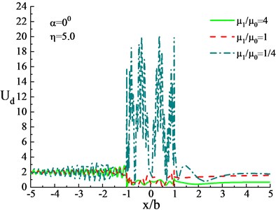
a)0°
b)90°
Fig. 19Surface displacement under influence of different shear modulus ratios of heterogeneous hill and the lower medium (η= 10.0)
a)0°
b)90°
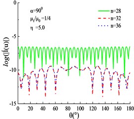
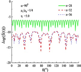
4.4. Referencing the influences of shear modulus ratio of the heterogeneous hill and lower medium on the displacement amplitude spectrum
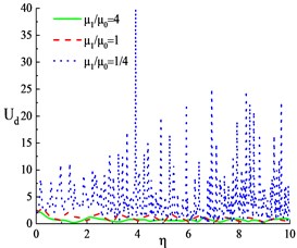
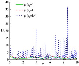
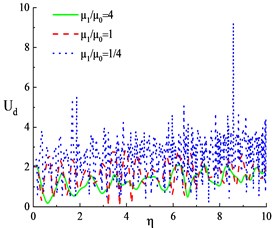
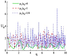
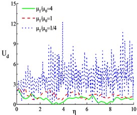
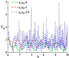
Figs. 20-22 show the displacement amplitude spectrum at three positions of the hill surface (top, left corner, and right corner), in which is the ratio of the shear modulus of the heterogeneous hill to the adjacent medium, is the incidence angle of the wave, and is the dimensionless frequency.
Fig. 20Displacement amplitude spectrum at the central point of the hill surface
a)0°
b)45°
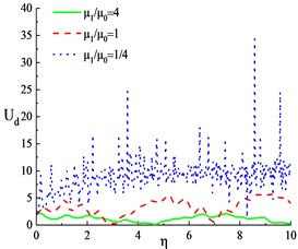
c)90°
Fig. 21Displacement amplitude spectrum at the left corner of the hill surface
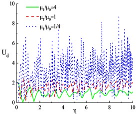
a)0°
b)45°
c)90°
Fig. 22Displacement amplitude spectrum at the right corner of the hill surface
a)0°
b)45°
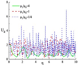
c)90°
The data from Figs. 20-22 show the surface displacement of the soft hill surface differs from that of the homogeneous and hard hill as follows:
(1) On the ground fixed observation point, in the case of homogeneous and hard conditions, the displacement amplitude of the surface changes with the frequency as a smooth curve, while the amplitude of the surface displacement of the soft hill changes with frequency as a non-smooth curve. As the hill topography gets softer, the fluctuation is more severe, implying that softer hill is more sensitive to the incident wave frequency.
(2) The soft hill area has a strong amplification effect on the upper surface motion, while the hard hill has a reducing effect on the ground motion. In addition, as the frequency increases, the amplitude of the surface displacement increases, with the maximum value tending to appear near 4.
As is shown in Fig. 20, in the amplitude spectrum of the surface displacement of the hill top point under the normal wave (90°), the maximum displacement amplitude of the top point of the homogeneous hill is 3.1, when the average displacement amplitude in the range of (the arithmetic mean of in the range of ) is 2.1. The maximum displacement amplitude of the soft hill top is 40 when and the average displacement amplitude in the range of is 7.8. Compared with the homogeneous conditions, these values are 13 and 3.7 times higher, respectively.
5. Conclusions
An improved wave function method is used innovatively for an incident SH wave in a half-space heterogeneous hill. The results show that the displacement and stress residual is so small along the entire boundary, including the corner points, and can be ignored. The solution is effective for high-frequency waves because of the high calculation accuracy. The frequency is calculated to be 10 in this paper, it is possible to study the characteristics of surface displacement at high frequencies. The medium hardness of hill topography has a great influence on the surface motion. Compared with the homogeneous hill, the surface displacement of the soft hill significantly increases, and the hard hill weakens the surface motion. It is suggested that seismic measures should be strengthened for engineering applications near the soft hill.
References
-
Abramowitz M., Stegun I. A. Handbook of Mathematical Functions, with Formulas, Graphs, and Mathematical Tables. Dover, New York, 1972.
-
Gutenberg B. Effect of ground on earthquake motion. Bulletin of the Seismological Society of America, Vol. 47, Issue 3, 1957, p. 221-250.
-
Kanai K., Suzuki T. Relation between the property of building vibration and the nature of ground (observation of earthquake motion at actual buildings). Earthquake Research Institute, Vol. 31, Issue 1, 1953, p. 305-316.
-
Kanai K., Suzuki T., Yoshizawa S. Relation between the property of building vibration and the nature of ground (observation of earthquake motion at actual buildings) III. Earthquake Research Institute, Vol. 34, Issue 1, 1955, p. 61-86.
-
Kanai K., Tanaka T., Yoshizawa S. Comparative studies of earthquake motions on the ground and underground (multiple reflection problem). Bulletin of the Earthquake Research Institute, Vol. 37, 1958, p. 53-87.
-
Tsai N. C. Influence of Local Geology on Earthquake Ground Motion. Ph.D., Thesis, 1969.
-
Trifunac M. D. Surface motion of a semi-cylindrical alluvial valley for incident plane SH wave. Bulletin of Seismological and Society of America, Vol. 61, Issue 6, 1971, p. 1755-1770.
-
Trifunac M. D. Scattering of plane SH wave by a semi-cylindrical canyon. Earthquake Engineering and Structural Dynamics, Vol. 1, Issue 3, 1973, p. 267-281.
-
Wong H. L., Trifunac M. D. Surface motion of a semi-elliptical alluvial valley for incident plane SH waves. Bulletin of the Seismological Society of America, Vol. 64, Issue 5, 1974, p. 1389-1408.
-
Wong H. L., Trifunac M. D. Scattering of plane SH waves by a semi-elliptical canyon. Earthquake Engineering and Structural Dynamics, Vol. 3, Issue 2, 1974, p. 157-169.
-
Liang J. W., Luo H., Lee V. W. Scattering of plane SH waves by a circular arc hill with a circular tunnel. Acta Seismologica Sinica, Vol. 17, Issue 5, 2004, p. 549-563.
-
Lee V. W. On deformations near circular underground cavity subjected to incident plane SH waves. Proceedings of the Symposium for Applications of Computer Methods in Engineering, Los Angeles, 1977, p. 951-961.
-
Lee VW., Luo H., Liang J. W. Anti-plane (SH) waves diffraction by a semi-circular cylindrical hill revisited: an improved accurate wave series analytic solution. Journal of Engineering Mechanics, ASCE, Vol. 132, Issue 10, 2006, p. 1106-1114.
-
Yuan X., Men F. L. Scattering of plane SH waves by a semi-cylindrical hill. Earthquake Engineering and Structural Dynamics, Vol. 21, Issue 12, 1992, p. 1091-1098.
-
Yuan X., Liao Z. P. Surface motion of a cylindrical hill of circular-arc cross-section for incident plane SH waves. Soil Dynamics and Earthquake Engineering, Vol. 15, Issue 3, 1996, p. 189-199.
-
Yuan X., Liao Z. P. Scattering of plane SH waves by arbitrary circularly raised topography. Earthquake Engineering and Engineering Vibration, Vol. 2, 1996, p. 1-13.
-
Vincent W., Lee., Luo H., Liang J. W. Antiplane (SH) Waves diffraction by a semicircular cylindrical hill revisited: an improved analytic wave series solution. Journal of Engineering Mechanics, Vol. 132, Issue 10, 2006, p. 1106-1114.
-
Vincent W., et al. Diffraction of anti-plane SH waves by a semi-circular cylindrical hill with an inside concentric semi-circular tunnel. Earthquake Engineering and Engineering Vibration, Vol. 3, 2004, p. 249-262.
-
Li Y. L., Yuan X., Sun R. Out of plane dynamic response of a heterogeneous hill in half space: the closed-form solution. Earthquake Engineering and Engineering Vibration, Vol. 25, Issue 3, 2005, p. 1-5.
-
Tsaur D. H., Chang K. H. Scattering and focusing of SH waves by a convex circular-arc topography. Geophysical Journal of the Royal Astronomical Society, Vol. 177, Issue 1, 2009, p. 222-234.
-
Tsaur D. H. Scattering and focusing of SH waves by a lower semi-elliptic convex topography. Bulletin of the Seismological Society of America, Vol. 101, Issue 5, 2011, p. 2212-2219.
-
Amornwongpaibun A., Luo H., Lee V. W. Scattering of anti-plane (SH) waves by a shallow semi-elliptical hill with a concentric elliptical tunnel. Journal of Earthquake Engineering, Vol. 20, Issue 3, 2016, p. 20.
-
Liu Z., Zhang H., Cheng A., et al. Seismic interaction between a lined tunnel and a hill under plane SV waves by IBEM. International Journal of Structural Stability and Dynamics, Vol. 19, Issue 2, 2018, p. 247-293.
-
Pao Y. H., Mow C. C., Achenbach J. D. Diffraction of elastic waves and dynamic stress concentrations. Journal of Applied Mechanics, Vol. 40, Issue 4, 1973, p. 872.
-
Lee V. W., Cao H. Diffraction of SV waves by circular cylindrical canyons of various depths. Journal of Engineering Mechanics, Vol. 11, Issue 8, 1989, p. 445-456.
-
Lee V. W., Karl J. Diffraction of SV waves by underground, circular, cylindrical cavities. Soil Dynamics and Earthquake Engineering, Vol. 11, Issue 8, 1992, p. 445-456.
-
Lee V. W., Karl J. Diffraction of elastic plane P waves by circular, underground unlined tunnels. European Earthquake Engineering, Vol. 6, Issue 1, 1993, p. 29-36.
-
Lee V. W., Wu X. Application of the weighted residual method to diffraction by 2-D canyons of arbitrary shape: I. Incident SH waves. Soil Dynamics and Earthquake Engineering, Vol. 13, Issue 5, 1994, p. 365-373.
-
Lee V. W., Wu X. Application of the weighted residual method to diffraction by 2-D canyons of arbitrary shape: Ⅱ. Incident P, SV, and Rayleigh waves. Soil Dynamics and Earthquake Engineering, Vol. 13, Issue 5, 1994, p. 355-364.
About this article

This work was supported by the Tianjin Research Program of Application Foundation Advanced Technology (17JCYBJC21700), the National Natural Science Foundation of China under grants (51878108), the key projects of Tianjin science and technology support program (17YFZCSF01140), and Tianjin Municipal Science and Technology Bureau (19PTZWHZ 00080).
