Abstract
The traditional method of fundamental solution (T-MFS) is known as an effective method for solving the scattering of elastic waves, but the T-MFS is inefficient in solving large-scale or broadband frequency problems. Therefore, in order to improve the performance in efficiency and memory requirement for treating practical complex 2-D broadband scattering problems, a new algorithm of fast multi-pole accelerated method of fundamental solution (FM-MFS) is proposed. Taking the 2-D scattering of SH waves around irregular scatterers in an elastic half-space as an example, the implementation steps are presented in detail. Based on the accuracy and efficiency verification, the FM-MFS is applied to solve the broadband frequency scattering of plane SH waves around group cavities, inclusions, a V-shaped canyon and a semi-elliptical hill. It shows that, compared with T-MFS, the FM-MFS has great advantages in reducing the consumed CPU time and memory for 2-D broadband scattering. Besides, the FM-MFS has excellent adaptability both for broad-frequency and complex-shaped scattering problems.
1. Introduction
The scattering of elastic waves is an attractive and significant topic in many fields such as in earthquake engineering, geophysics, civil engineering, etc. In general, the calculation methods for the wave scattering include the analytical methods and numerical methods. The analytical methods are mainly referred to the wave function expansion methods [1-8]. The numerical methods include finite difference methods (FDM) [9, 10], finite element methods (FEM) [11, 12], boundary element methods (BEM) [13-20], and more works can be found in a review by Sanchez-Sesma et al. [21] and by Manolis and Dineva [22].
Among different boundary-type methods, the method of fundamental solution (MFS) not only reduces the dimension of problem and automatically satisfy the boundary conditions at infinite, but also is a meshless method. In the MFS, the approximate solution of the partial differential equation is constructed by the linear combination of a series of Green’s functions. In order to avoid singularities, the fictitious wave sources are placed at some distance to the physical boundaries of scatters. The densities of the fictitious sources are firstly obtained by the boundary integral equations discretized through boundary collocation points. So, the MFS can also be regarded as a special indirect boundary integral equation method which is very similar to the Trefftz method [23].
Due to the excellent numerical accuracy and simplicity of usage, the MFS (also named indirect boundary integral equation method) has been widely applied in the field of wave scattering in an elastic medium [24-32]. However, just as other boundary-type numerical methods, the MFS suffers a large difficulty in treating large-scale models. A significant weakness of MFS is that the calculation efficiency of solving high-DOF problem (such as large scale, broadband frequency or multi-body scattering) is seriously affected by its dense characteristic of the equation matrix. Chen et al. [33] greatly improved the computational efficiency of MFS using a sparse storage method, but the method still has some limitations to overcome this weakness. Some researchers tried to combine the FMM with the MFS in recent years. In essence, The FMM separates source points from collocation points of the kernel function expressions to change the Green’s function calculation from one-to-one interaction to group-to-group interaction. Then the FMM can substantially reduce the memory requirement and improve the computational efficiency [34-36]. The FM-MFS has been developed for solving many large-scale practical engineering problems [37-39]. The memory of MFS can be reduced to () by the latest development of FMM, and the computation amount is reduced to () order. It should be noted that the references mentioned above are all about the potential problems, the static analysis or the acoustic simulation. According to the author’s knowledge, the FM-MFS applied to elastic waves scattering problem in solid and the corresponding research are still rare at present. It is worth mentioned that there have been some reports related to the FMM-BEM [40, 41], but the associated BEM is largely different from the meshless MFS.
In this paper, in order to overcome the disadvantage of traditional MFS and solve large-scale elastic wave-motion problems in a half-space, a new algorithm of the FM-MFS is proposed and validated. The method is based on the single layer potential theory, and introduces the fast multi-pole expansion to construct the Green’s functions matrix. The virtual source density is obtained through GMRES iteration, of which the solving process is direct, and it is convenient for numerical implementation. Taking the 2-D scattering of SH waves around an irregular scatter in an elastic half-space as an example, the implementation steps are presented in detail, and then several typical examples indicate the excellent accuracy and efficiency of the method. Finally, the scattering of plane SH waves by randomly distributed cavity or inclusion group, by a canyon and hill topography in a half-space are solved and discussed.
2. The traditional MFS
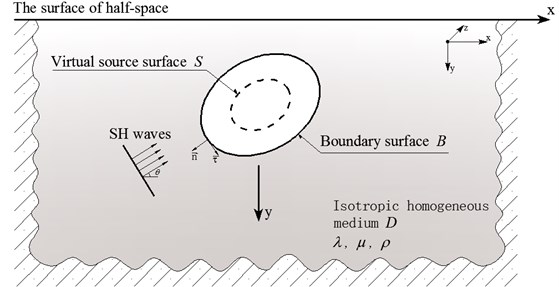
Fig. 1 shows the calculation model. Assuming the incident waves are plane SH waves , are the two parameters of Lame constant, and is the medium density is the shear wave number, defined as , where is the circular frequency of seismic waves, is the velocity of shear waves. The steady-state motion equation in isotropic homogeneous medium is as follows:
where is the anti-plane displacement. Note that the time factor is omitted in Eq. (1) and thereafter.
According to numerical experience, the wave sources can be placed within 0.4-0.6 times of the relevant radius of the scatterer for low frequency waves (non-dimensional frequency , is the scatterer radius); while for high frequency wave (), the wave sources should better be placed within 0.7-0.9 times of the relevant radius of the scatterer.
Firstly, the wave field should be separated. And the total displacement field and the stress field in the elastic half-space can be expressed as:
where and are anti-plane displacement and shear stress of the free-field under incident plane SH waves. and are displacement and stress of the scattered wave field. The scattered field in is constructed by the virtual sources . Consequently, the boundary condition can be written as:
According to the single layer potential theory, virtual sources on produce the scattered field in the half-space. Related displacement and stress are expressed as follows:
In which , . is the strength of shear-wave line source corresponding to position on virtual sources . and are the displacement Green's functions and stress Green’s functions in the elastic half-space which can be introduced as:
where is the Hankel function of the second kind with order 0, and are the unit normal vectors, , . As is shown in Fig. 2, is the mirror point of .
Fig. 1The calculation model
Set observed points on boundary , and points on the virtual sources . We choose the unit center physical quantity instead of unit physical quantity, then the linear system of equations become:
Eq. (9) can be reformatted as:
where is the dense non-symmetric coefficients matrix, is the densities of fictitious sources on virtual boundary. denotes the response related to the free field on the boundary.
To speed up the calculation, a new algorithm of fast multi-pole fundamental solution method (FM-MFS) is presented. This method can greatly shorten the calculation time and reduce the needed memory. Combining General Minimize Residual Methods (GMRES) [42] with the fast multi-pole expansion technique [43], large-scale or high-frequency scattering of elastic waves can be solved effectively.
3. The new fast multi-pole for MFS
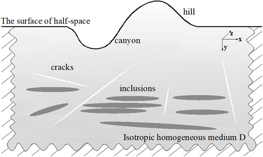
In traditional method of fundamental solution, it is difficult to calculate the approximate solutions for large-scale or high-frequency problems using the GMRES iterative algorithm. As shown in Fig. 2, consider a large number of cracks and inclusions existing in the actual complex terrain. For such problems, integration equations with high DOFs need to be calculated.
Fig. 2The calculation model of large-scale or multi-scatter problem
To solve the Eq. (10), the large coefficients matrix is needed to storage. But the memory requirement is so high that this algorithm loses its practical value. The tree structure is used as the main storage and computing object in the FM-MFS, which can expand and transfer the kernel function. By taking the GMRES iterative algorithm, we can multiply and the tree structure instead of the large coefficients matrix . Then results are obtained by controlling iterative precision. Different kernel functions apply to different expansion methods. In this paper, the plane wave expansion theorem is taken to expand the kernel function in Eq. (7) as:
where, and is the center of multi-pole expansion, is the angle between and axis, , , and the number of truncated.
Therefore, it can be shown that Eq. (6) can be rewritten as:
In which and are the multi-pole moments and can be expressed as:
and in Eq. (15) are only related to and . Furthermore, it needs to calculate only once for arbitrary collocation points for satisfying conditions.
Fig. 3Related points for FM-MFS expansion
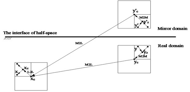
As shown in Fig. 3, new multi-pole moments can be obtained when points for expansion moved from , to , . The M2M transfer can be written as:
From equations above, the multi-pole moments do not need to be calculated again, but the calculated coefficient should be translated into new multi-pole moments.
Assuming a point ,which is close to point , satisfying . And the local expansion to Eq. (15) can be expressed as:
where, and can be obtained by M2L transformation of multi-pole moments and , as follows:
Finally, the local expansion transmission of L2L can be expressed as:
Take the scattering of SH waves by a cavity in a half space as an example, the implementation procedures is listed as follows.
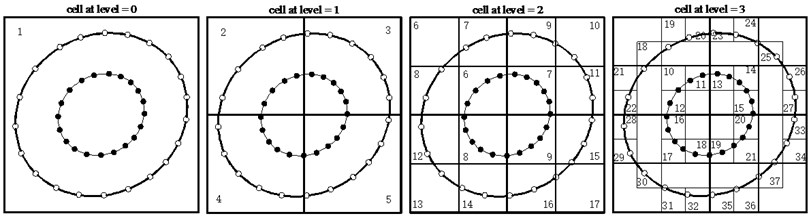
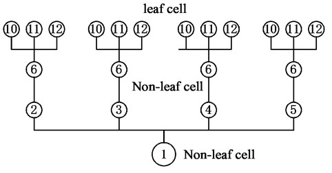
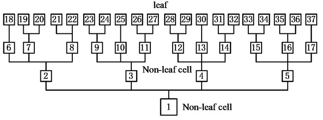
Step 1. Discretization. Discrete the boundary and , the same as in the T-MFS, and then automatically generate the adaptive tree structure (See Fig. 4).
Fig. 4The adaptive tree structure
a) Construction of quad-tree structure
b) Virtual wave source point
c) Boundary point
Step 2. Upward pass. Translate information from the source points, to the leaf cells. Eq. (16) and Eq. (17) are expanded in the center of leaves to generate multi-pole expansion moments. And then the multi-pole expansion point can be moved to the corresponding parent cell (M2M). Eq. (18) and Eq. (19) constitute the transfer relationship. In this step, transfer can be repeated several times to the parent cells. If satisfying the accuracy conditions, upward pass can be carried out ( 2) (see Fig. 4(a), (b)).
Step 3. Downward pass. The multi-pole expansion moments of each level cell on the tree structure can be transferred into corresponding local expansion moments (M2L), and Eq. (21) and Eq. (22) can be applied to build this relationship. Transfer the local expansion moments of each level cell in the tree structure to the leaf cell by using Eq. (23). So far, all local expansion moments at leaf cells can be translated to the boundary points through local expansion. The total expansion and transfer processes are completely given.
Step 4. Near-source calculation. The contributions of the near field virtual source points can be calculated by the T-MFS.
Step 5. Iterations. Update the unknown vector in the system until the solution converges within a given tolerance using the GMRES solver.
4. Accuracy and computational efficiency
Taking the wave scattering around a cavity in half-space as an example, the accuracy and numerical stability of FM-MFS are tested and compared with analytical solution [44]. As is shown in Fig. 1, assuming the radius of the circular hole is , the number of collocation points on boundary is 2000 (), the embedment depth is , shear modular is , surface width is , the incident angle of SH waves is 90°,and the dimensionless frequency is 0-20, the expansion terms10, the iterative error is 10-3. Fig. 5 illustrates the displacement amplitude on the surface by FM-MFS compared with that by analytical solution. Table 1 shows the displacement amplitude on the surface center for the vertical incident SH waves ( 90°) under different degrees of freedom. The comparison illustrates that the results by FM-MFS agree well with those by analytical solution, and have good numerical stability.
Fig. 5Comparisons between the displacement amplitude on the surface by FM-MFS and that of analytical solution
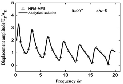
Table 1Numerical stability of displacement amplitudes
DOFs | Displacement amplitude ( 0, ) | |
FM-MFS | T-MFS | |
100 | 2.706531 | 2.706835 |
500 | 2.706502 | 2.706782 |
1000 | 2.706532 | 2.706774 |
5000 | 2.706553 | 2.706772 |
10000 | 2.706521 | 2.706772 |
Exact | 2.706772 | – |
To test the efficiency of FM-MFS, the scattering of plane SH wave is considered by a cylindrical cavity in an elastic half space. Model parameters are as above and the DOFs increase from 100to 50000. As shown in Fig. 6, complexity of the T-MFS is about total CPU time, and the calculation time has reached 9147s when the DOFs are only 10000. However, the complexity of the FM-MFS is , and the calculation time is only 30 s when the DOFs reach 50000. Near field calculation becomes unnecessary due to low frequency, sources with small radius and the tree structure with fine mesh. Fig. 7 illustrates comparison of memory between T-MFS and the present FM-MFS. The storage requirement of T-MFS increases rapidly with the increase of DOFs. When the DOFs reaches 10000, the memory is more than 1.5 GB. However, the required memory will be greatly reduced when using the FM-MFS. For 50000 DOFs, the occupied memory is only 66 MB for the FM-MFS. Therefore, compared with the T-MFS, both the CPU time and memory performance are greatly improved by FM-MFS. These advantages speed up fast solution of 2D large-scale or broadband scattering problem of elastic waves.
Fig. 6Total CPU time used to solve the wave scattering
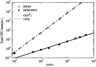
Fig. 7Total memory used to solve the wave scattering
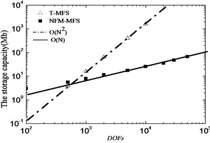
Fig. 8The surface displacement amplitude for incident SH waves
a)
b)
c)
d)
5. Numerical examples
5.1. The scattering of SH wave by cavities group
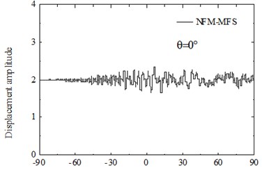
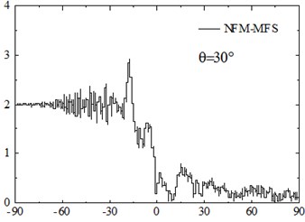
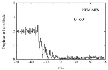
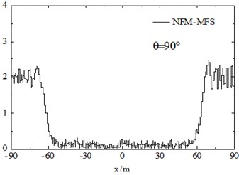
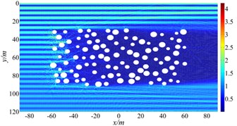
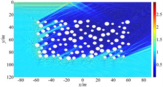
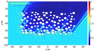
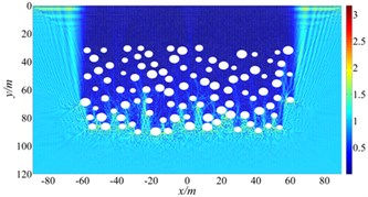
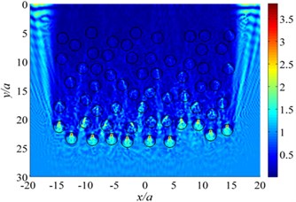
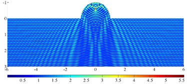
The FM-MFS can be used to calculate the scattering of seismic waves for shallow underground cavities distributed randomly in a half space. 30 m under the surface of the ground, 100 random cavities are established to simulate fracture within the scope of 60 m×120 m. Radiuses of circular cavities are ranging from 1.5 m to 3 m and 10,00 boundary points are set on the surface of each cavity. The total number of DOFs reaches 105. The dimensionless frequency is set as 150-300. The iterative error is 10-3, and 0°, 30°, 60°,90°. Fig. 8 shows the surface displacement amplitude of cavities. The consumed CPU time is 803 s and the storage of main matrix is 2011 MB.
Numerical results show that random cavities have significant effect on the scattering of SH waves. As shown in Fig. 8, for vertical incidence of the SH waves, the displacement amplitudes of the surface is greatly decreased, for example, the displacement amplitude near 0 is only about 0.1. For the oblique incidence of SH waves, there is obvious amplification effect on the incident side and the amplitude close to two times of free-field displacement, but the displacement on the side behind the wave is significantly decreased. Therefore, random cavities group has a strong “barrier effect” on incident wave. Fig. 9 shows displacement amplitudes around the cavities under SH wave incidence. It can be seen that the coherence effect of scattering waves among cavities is very strong. The displacement amplitude reached more than 4.0 when the incident wave is close to the horizontal incidence. For the vertical incidence, the displacement amplitude around cavities is more than 1.5 times of the free field displacement amplitude. Therefore, for the safety of tunnel and underground pipeline engineering, crossing the cavities zone should be avoided, especially in the side of the incident wave.
Fig. 9The displacement amplitude around the cavities group for incident SH waves (ka= 150-300)
a) 0°
b) 30°
c) 60°
d) 90°
5.2. The scattering of SH wave by inclusions group
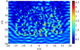
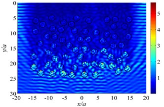
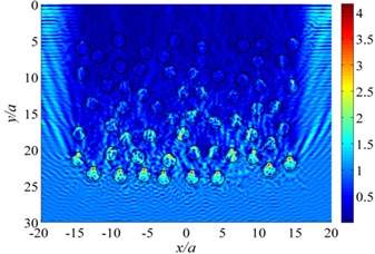
The scattering of plane SH wave is considered by inclusions group in a 30×40 domain, where is radius of the inclusion. Fig. 10 illustrates the results of displacement amplitude with variation of incident wave frequency. Calculation parameters are set to be: density ratio between the inclusion and the half space 2/3, Poisson’s ratio 0.25, 0.30. DOFs = 61000. The tolerance for convergence is set to 10-3. In this calculation, the CPU time is about 205 seconds and the memory usage is about 1.3 GB, 0.5, 1.0, 2.0, 5.0.
Assume incident plane waves propagating along -direction. Fig. 10 plots the contours of displacement amplitude around inclusions group under SH wave incidence for 0.5, 1.0, 2.0, 5.0, and shear-wave speed ratio 1/2. It demonstrates that the scattering effect of elastic wave by inclusions seems more obvious as the frequency increases. For 1.0, the normalized displacement amplitude reaches up to 5.3, more than five times that of incident wave, which is mainly due to coherent effects of multiple scattering wave among inclusions group.
Fig. 10The displacement amplitude around the inclusions group for incident SH waves (θ= 0°)
a) 0.5
b) 1.0
c) 2.0
d) 5.0
5.3. The scattering of SH wave by a V-shaped canyon
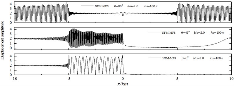
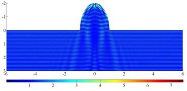
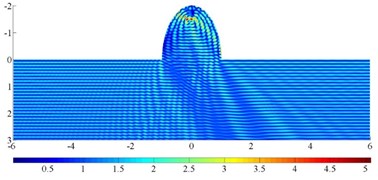
Displacement amplitude on the surface of a V-shaped canyon under incident high-frequency SH waves are shown in Fig. 12 and Fig. 13. The discrete number of canyon surface is 200359, the calculation time is about 732 s, and the consumed memory is 2.4 GB. The parameters are set to be: the wideness of the V-shaped canyon 2 km, the incident frequency 20 Hz, the shear wave velocity 400 m/s, the dimensionless frequency 100, / 1.0, 2.0, and the iterative error 10-6, incident angle 0°, 45°, 90° (Fig. 11).
Fig. 11Diffraction of plane SH waves by a V-shaped canyon
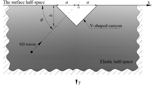
Numerical results show that the left of the canyon appears significant displacement amplification effect with the incidence of high-frequency SH waves (left incidence), about twice the size of free-field displacement amplitude ratio. And the right side shows a very long “shadow zone”, indicating canyon has a shielding effect under the incident waves. Under oblique incidence, the amplification effect of canyon is particularly remarkable. With vertical incidence, the displacement amplitude at the corner of the V-shaped canyon is about 3.0, 50 % more than the free-field displacement. For high frequency wave incidence, the displacement response varies widely even in a small spatial scale, and displacement response of the canyon is violent on the side of the incident wave. Thus, to analyze the seismic response of bridge or dam located in canyon, the amplification effect of seismic waves scattering and uneven spatial distribution should be considered, and special attention should be paid to the high-frequency wave of oblique incidence. Calculation of the seismic responses of an engineering structure in a canyon may produce large error if using a uniform seismic input.
Fig. 12The surface displacement amplitude around a V-shaped canyon for incident SH waves (b/a= 1.0)
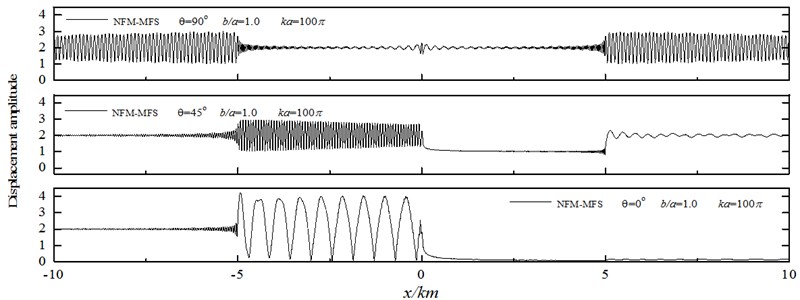
Fig. 13The surface displacement amplitude around a V-shaped canyon for incident SH waves (b/a= 2.0)
5.4. The scattering and focusing of SH wave by a semi-elliptical hill
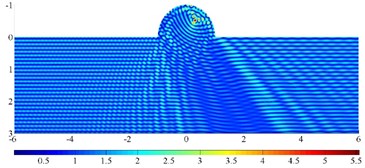
Fig. 14 illustrates the contour of displacement amplitude around a semi-elliptical hill under incident high-frequency SH waves. The parameters are set to be: the wideness of the hill 1km, the incident frequency 5 Hz, the shear wave velocity 500 m/s, the dimensionless frequency 10, / 1.0, 2.0,5.0 and the iterative error 10-6, incident angle 60°, 90°.
The results show that the seismic response characteristics of the hill are significantly dependent on the incident wave angle and the aspect ratio of the hill. For the high steep hill, the focal effect of the seismic wave near the top is the most significant, such as for / 5.0, the displacement peak reaches 8.3, and the corresponding semi-circular hill displacement peak is 5.5. As for the spatial distribution feature, displacement amplification area is widely distributed on the semi-circular hill, but is mainly concentrated in the hill surface for the high steep hill. Thus, in actual violent earthquakes, the damage of high and steep slopes is usually serious. In addition, due to the coherence effect of the surface creeping wave, reflected wave and direct wave, the wave crest and wave node of the displacement response appear alternately on the surface of the hill, which is more significant for a high-steep hill. Considering the change of incident angle, the focusing position is also greatly shifted for oblique incidence, and the range of displacement amplification of a high and steep hill is enlarged. Correspondingly, the peak displacement is smaller than that of vertical incidence. The similar focusing phenomenon has also been observed by Chen et al. [45]. Note that the accurate solution to the high-frequency wave scattering by a high-steep hill also illustrate excellent adaptability of the FM-MFS for treating practical problems.
Fig. 14The surface displacement amplitude around a semi-elliptical hill for incident SH waves (ka= 10π)
a)/ 1, 90°
b)/ 1, 60°
c)/ 2, 90°
d)/ 2, 60°
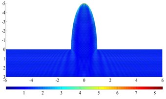
e)/ 5, 90°
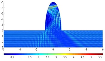
f)/ 5, 60°
6. Conclusions
Combined with the new fast multi-pole expansion technique, the large-scale or high-frequency scattering problem of SH waves by 2-D superficial irregularities or heterogeneity in a solid half-space is solved by the proposed FM-MFS. By using the plane wave expansion of SH wave potential function, requirement of the CPU time and memory of multi-pole and local expansion is substantially reduced. The accuracy of this method is verified by comparing with exact solution. It is demonstrated that the FM-MFS can effectively solve practical complex scattering problem. Numerical results also show several interesting scattering characteristics of the high-frequency elastic waves generated by a V-shaped canyon, a semi-elliptical hill and inclusions (cavities) group. All these numerical examples indicate that the proposed FM-MFS has favorable numerical accuracy and efficiency, providing a novel effective method for the simulation of large-scale and high-frequency wave propagation problems for arbitrary-shaped scatters.
References
-
Trifunac M. D. Scattering of plane SH wave by a semi-cylindrical canyon. Earthquake Engineering and Structural Dynamics, Vol. 1, Issue 3, 1973, p. 267-281.
-
Todorovska M. I., Lee V. W. A note on scattering of Rayleigh waves by shallow circular canyons: analytical approach. Bulletin of the Indian Society of Earthquake Technology, Vol. 28, Issue 2, 1991, p. 1-16.
-
Yuan X. M., Liao Z. P. Scattering of plane SH waves by a cylindrical alluvial valley of circular-arc cross section, Earthquake Engineering and Engineering Vibration, Vol. 24, Issue 10, 1995, p. 1303-1313.
-
Li W. H., Zhao C. G. Scattering of elastic waves by cylindrical scatterers in saturated porous medium. Soil Dynamics and Earthquake Engineering, Vol. 25, Issue 12, 2005, p. 981-995.
-
Liang J. W., Ba Z. N., Lee V. W. Diffraction of plane SV waves by a shallow circular-arc canyon in a saturated poroelastic half-space. Soil Dynamics and Earthquake Engineering, Vol. 26, Issue 6, 2006, p. 582-610.
-
Gao Y. F., Zhang N., Li D., Liu H., Cai Y., Wu Y. Effects of topographic amplification induced by a U-shaped canyon on seismic waves. Bulletin of the Seismological Society of America, Vol. 102, Issue 4, 2012, p. 1748-1763.
-
Lee V. W., Zhu G. A note on three-dimensional scattering and diffraction by a hemispherical canyon – I: Vertically incident plane P-wave. Soil Dynamics and Earthquake Engineering, Vol. 61, Issue 2, 2014, p. 197-211.
-
Zhang N., Gao Y. F., Yang J., Xu C. J. An analytical solution to the scattering of cylindrical SH waves by a partially filled semi-circular alluvial valley: near-source site effects. Earthquake Engineering and Engineering Vibration, Vol. 14, Issue 2, 2015, p. 189-201.
-
Olsen K. B., Pechmann J. C., Schuster G. T. Simulation of 3D elastic wave propagation in the Salt Lake Basin. Bulletin of the Seismological Society of America, Vol. 85, Issue 6, 1995, p. 1688-1710.
-
Lee S. J., Chen H. W., Huang B. S. Simulations of strong ground motion and 3D amplification effect in the Taipei Basin by using a composite Grid finite-difference method. Bulletin of the Seismological Society of America, Vol. 98, Issue 3, 2008, p. 1229-1242.
-
Padovani E., Priolo E., Seriani G. Low and high order finite element method: experience in seismic modeling. Journal of Computational Acoustics, Vol. 2, Issue 4, 1994, p. 371-422.
-
Chen G. X., Jin D. D., Zhu J., Shi J., Li X. J. Nonlinear analysis on seismic site response of Fuzhou basin, China. Bulletin of the Seismological Society of America, Vol. 105, 2015, p. 928-949.
-
Gonsalves I. R., Shippy D. J., Rizzo F. J. Direct boundary integral equations for elastodynamics in 3-D half-spaces. Computational Mechanics, Vol. 6, Issue 4, 1990, p. 279-292.
-
Sanchez-Sesma F. J., Luzon F. Seismic response of three-dimensional alluvial valleys for incident P, S, and Rayleigh waves. Bulletin of the Seismological Society of America, Vol. 85, Issue 1, 1995, p. 269-284.
-
Pointer T., Liu E., Hudson J. A. Numerical modelling of seismic waves scattered by hydrofractures: application of the indirect boundary element method. Geophysical Journal of the Royal Astronomical Society, Vol. 135, Issue 1, 1998, p. 289-303.
-
Karabulut H., Ferguson J. F. An analysis of the indirect boundary element method for seismic modelling. Geophysical Journal of the Royal Astronomical Society, Vol. 147, Issue 1, 2001, p. 68-76.
-
Tadeu A., Mendes P. A., António J. 3D elastic wave propagation modelling in the presence of 2D fluid-filled thin inclusions. Engineering Analysis with Boundary Elements, Vol. 30, Issue 3, 2006, p. 176-193.
-
Dineva P. S., Wuttke F., Manolis G. D. Elastic wave scattering and stress concentration effects in non-homogeneous poroelastic geological media with discontinuities. Soil Dynamics and Earthquake Engineering, Vol. 41, 2012, p. 102-118.
-
Chen W., Zhang J. Y., Fu Z. J. Singular boundary method for modified Helmholtz equations. Engineering Analysis with Boundary Elements, Vol. 44, 2014, p. 112-119.
-
Fu Z. J., Chen W., Chen J. T., Qu W. Z. Singular boundary method: Three regularization approaches and exterior wave applications. Computer Modeling in Engineering and Sciences, Vol. 99, Issue 5, 2014, p. 471-443.
-
Sanchez-Sesma F. J., Palencia V. J., Luzon F. Estimation of local site effects during earthquakes: an overview. ISET Journal of Earthquake Technology, Vol. 39, Issue 3, 2002, p. 167-193.
-
Manolis G. D., Dineva P. S. Elastic waves in continuous and discontinuous geological media by boundary integral equation methods: A review. Soil Dynamics and Earthquake Engineering, Vol. 70, 2015, p. 11-29.
-
Chen J. T., Lee Y. T., Yu S. R., Shieh S. C. Equivalence between the Trefftz method and the method of fundamental solution for the annular Green’s function using the addition theorem and image concept. Engineering Analysis with Boundary Elements, Vol. 33, Issue 5, 2009, p. 678-688.
-
Wong H. L. Effect of surface topography on the diffraction of P, SV, and Rayleigh waves. Bulletin of the Seismological Society of America, Vol. 72, Issue 4, 1985, p. 1167-1183.
-
Dravinski M., Mossessian T. K. Scattering of plane harmonic P, SV, and Rayleigh waves by dipping layers of arbitrary shape. Bulletin of the Seismological Society of America, Vol. 77, Issue 1, 1987, p. 212-235.
-
Kondapalli P. S., Shippy D. J., Fairweather G. The method of fundamental solutions for transmission and scattering of elastic waves. Computer Methods in Applied Mechanics and Engineering, Vol. 96, Issue 2, 1992, p. 255-269.
-
Luco J. E., Barros F. C. P. D. Dynamic displacements and stresses in the vicinity of a cylindrical cavity embedded in a half-space. Earthquake Engineering and Structural Dynamics, Vol. 23, Issue 3, 1994, p. 321-340.
-
Tadeu A., Godinho L., António J., Mendes P. A. Wave propagation in cracked elastic slabs and half-space domains – TBEM and MFS approaches. Engineering Analysis with Boundary Elements, Vol. 31, Issue 10, 2007, p. 819-835.
-
Tadeu A., António J., Godinho L. Defining an accurate MFS solution for 2.5D acoustic and elastic wave propagation. Engineering Analysis with Boundary Elements, Vol. 33, Issue 12, 2009, p. 1383-1395.
-
Lin J., Chen W., Sun L. Simulation of elastic wave propagation in layered materials by the method of fundamental solutions. Engineering Analysis with Boundary Elements, Vol. 57, 2015, p. 88-95.
-
Sun L., Chen W., Cheng H. D. Method of fundamental solutions without fictitious boundary for plane time harmonic linear elastic and viscoelastic wave problems. Computers and Structures, Vol. 162, 2016, p. 80-90.
-
Liu Z. X., Liang J. W., Wu C. Q. The diffraction of Rayleigh waves by a fluid-saturated alluvial valley in a poroelastic half-space modeled by MFS. Computers and Geosciences, Vol. 91, 2016, p. 33-48.
-
Chen C. S., Jiang X., Chen W., Yao G. Fast solution for solving the modified helmholtz equation with the method of fundamental solutions. Communications in Computational Physics, Vol. 17, Issue 3, 2015, p. 867-886.
-
Greengard L., Rokhlin V. A fast algorithm for particle simulations. Journal of Computational Physics, Vol. 135, Issue 2, 1997, p. 280-292.
-
Yao Z. H., Wang H. T. Boundary Element Methods. Higher Education Press, Bei Jing, 2009.
-
Cui X. B., Ji Z. L. Application of FMBEM to calculation of sound fields in sound-absorbing materials. Journal of Vibration and Shock, Vol. 30, Issue 8, 2011, p. 187-192.
-
Liu Y. J., Nishimura N., Yao Z. H. A fast multi-pole accelerated method of fundamental solutions for potential problems. Engineering Analysis with Boundary Elements, Vol. 29, Issue 11, 2005, p. 1016-1024.
-
Xu Q., Jiang Y. T., Zhang Z. J. Fast multi-pole VBEM for analyzing the effective elastic moduli of a sheet containing circular holes. Chinese Journal of Computational Mechanics, Vol. 27, Issue 3, 2010, p. 548-555.
-
Jiang X. R., Chen W., Chen C. S. A fast method of fundamental solutions for solving Helmholtz-type equations. International Journal of Computational Methods, Vol. 10, Issue 2, 2013, p. 292-299.
-
Chen Y. H., Chew W. C., Zeroug S. Fast multi-pole method as an efficient solver for 2D elastic wave surface integral equations. Computational Mechanics, Vol. 20, Issue 6, 1997, p. 495-506.
-
Chaillat S., Bonnet M., Semblat J. F. A new fast multi-domain BEM to model seismic wave propagation and amplification in 3-D geological structures. Geophysical Journal of the Royal Astronomical Society, Vol. 177, Issue 2, 2009, p. 509-531.
-
Saad Y., Schultz M. H. GMRES: A generalized minimal residual algorithm for solving nonsymmetric linear systems. Siam Journal on Scientific and Statistical Computing, Vol. 7, Issue 3, 1986, p. 856-869.
-
Nishimura N. Fast multi-pole accelerated boundary integral equation methods. Applied Mechanics Reviews, Vol. 55, Issue 4, 2002, p. 299-324.
-
Lee V. W. On deformations near a circular underground cavity subjected to incident plane SH waves, Proceedings of the Application of Computer Methods in Engineering Conference, Vol. 105, 1977, p. 952-962.
-
Chen J. T., Lee J. W., Shyu W. S. SH-wave scattering by a semi-elliptical hill using a null-field boundary integral equation method and a hybrid method. Geophysical Journal International, Vol. 188, Issue 1, 2012, p. 177-194.
Cited by
About this article

This work was supported in part by the National Natural Science Foundation of China (No. 51578372), and the Science and Technology Support Program Key Project of Tianjin (No. 17YFZCSF01140).
Mr. Zhongxian Liu formulated the overall research program and guided the preparation of code. Details as follows: Zhikun Wang was responsible for writing essays and programming code, data sorting and analysis was finished by Linping Guo and the code was prepared by Fengjiao Wu, additionally, Dong Wang is in charge of formula derivation and data management.
