Milling cutter condition reliability prediction based on state space model

2.1. Condition monitoring

Condition monitoring is of great importance in order to estimate the tool wear. Cutting force is used on condition estimation as it is directly related to wearing process. Our research aims to retrieve sufficient monitoring information of MC wear condition. It is in favour of cost reduction, implementation feasibility, and so on. As well, it is also not easy to implement the on-the-fly measurement of wearing capacity of MC in the actual production. Milling force, vibration signal, acoustic emission (AE) signal have been investigated used on MC wearing process. At present, the cutting force measurement is only used in the experimental study. But it is hard to be applied to the actual production for MC condition monitoring. In this research, AE signal is investigated on MC condition monitoring and fault diagnosis.

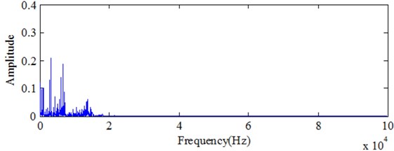
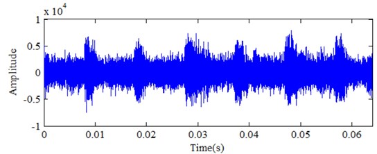
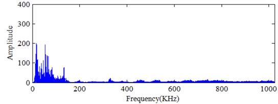
Milling test is conducted on the DONG YU JINGJI CMV- 850A machining center in Mold Center, Dalian University of Technology and the material is FV520B. FV520B is a special material for impeller production. Its high hardness keeps blade working in the designed condition. Choose domestic APOLL550 portable industrial PC and AEwin data acquisition software of PAC company for the acoustic emission signal data acquisition. The MC life experiment is carried in accelerated manner. The spindle speed is 1000 rpm, the cutting depth is 0.4 mm, and the feed rate is 400 mm/min. The acoustic emission signal sampling length is 512000 points and the sampling frequency $F_s$ is 2048 kHz. Samples are collected every 10 seconds and 240 sets of acoustic emission signals are collected before the cutter tool coming to the stage of failure. Fig. 1 presents the picture for the test-rig. In the experiment, cutting force and AE signal are monitored to determine the parameter for condition classification. Fig. 2 gives the picture for the comparison of MC in different working conditions. Which mean normal and wearing condition, respectively. Cutting force and AE are determined based on the experiment for different working conditions. Fig. 3 and Fig. 4 show the comparison for cutting force with time domain and frequency spectrum in different conditions. It is obvious with cutting force amplitude increase with wearing conditions. There is much difference between normal and serious wearing condition. It means that cutting force is highly related with wearing process. But it is not convenient to monitor in practical condition. AE signals are also obtained during the experiment. Fig. 5 and Fig.6 show the comparison for AE with time domain and frequency spectrum in different conditions. It can also determine that AE signal will increase with MC wearing process. Therefore, it can be used to demonstrate the wearing process. But further investigation should be carried on as there is much noise interference. Effectively feature extraction can improve the accuracy of pattern recognition. Therefore, characteristic parameters are investigated to determine the best one to demonstrate the wearing process.

Fig. 1Test rig

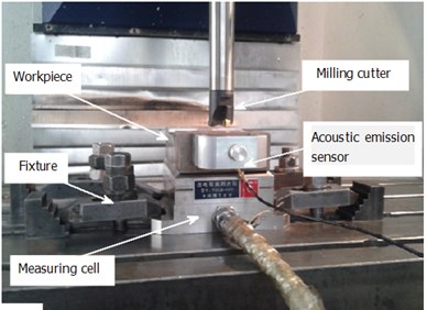
Fig. 2Picture for cutting tools in different conditions

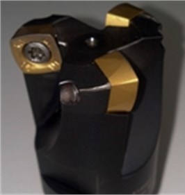
a) Intact condition

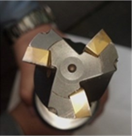
b) Wear condition

Fig. 3Signal analysis for cutting force in normal condition

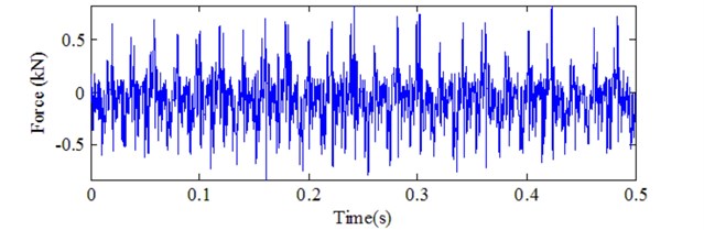
a) Time domain

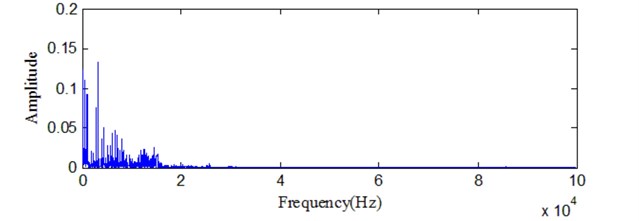
b) Frequency spectrum

2.2. Feature extraction

Root mean square (RMS) has been broadly used on machine condition estimation and reliability prediction. But it is not sensitive to some signals and further extraction is urgently needed. Many researchers have worked on the signal processing technology. Vibration signal processing and feature extraction have been intensively investigated in the last two decades, such as time domain analysis, frequency domain analysis, time-frequency domain analysis. With the development of the wavelet analysis in last three decades, it has been broadly used to process vibration signals and the effect is remarkable [15]. As the extension and development of wavelet transform, Wavelet Packet Decomposition (WPD) is multi-dimension process. Therefore, it has been investigated by many researchers.

Suppose there is a scaling space of limited energy signal $U_0^0$. Through wavelet packet transformation [16], $U_0^0$ is decomposed into several spaces in binary format. The iterative formula is:

Fig. 4Signal analysis for cutting force in seriously wearing condition

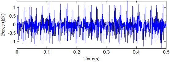
a) Time domain

b) Frequency spectrum

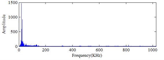
Fig. 5Signal analysis for AE in normal condition

a) Time domain

b) Frequency spectrum

In Eq. (1), $j$$(j\le 0)$ is decomposition level, $\oplus$ expresses orthogonal decomposition, $U_{j+1}^k$, $U_j^{2k}$, and $U_k^{2k+1}$ three closure spaces respectively corresponding wavelet function are:

When $n=0$, ${\psi }_0\left(t\right)$ is a scaling function $\phi \left(t\right)$ and ${\psi }_1\left(t\right)$is a wavelet basis function $\psi \left(t\right)$, $h\left(k\right)$ and $g\left(k\right)$ are discrete quadrature mirror filter coefficients. The signals in the space $U_j^{n-1}$ can be obtained by wavelet packet function ${\psi }_k^{j,n}\left(t\right)$ reconstruction, which is shown in Eq. (4):

Fig. 6Signal analysis for AE signal in seriously wearing condition

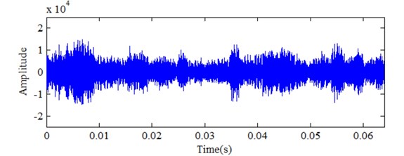
a) Time domain

b) Frequency spectrum

In Eq. (4), $D_k^{j,n}$ is wavelet packet coefficient, and it can be obtained by the following equation:

The wavelet packet function ${\psi }_{j,k}\left(t\right)$ is orthogonal basis function in $L^2\left(R\right)$, so the energy of $s_j^n\left(t\right)$ is:

The normalized wavelet packet energy is:

2.3. Correlation analysis for AE and force

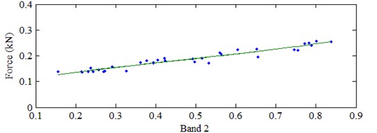
Zhong [15] did the correlation analysis on the related characteristics of acoustic emission signals and force signals with tool wear. The results show that acoustic emission characteristic is the same as force signal characteristic and it is highly correlated with tool wear. Fig. 10 provides different frequency energy bands distribution comparison at different conditions. The wearing condition is obvious larger than normal condition in the second frequency band. It also means that the second frequency band energy increases with MC degradation process. Fig. 7 gives the development trend for the wearing degradation with the second frequency band energy and cutting force. It is also the same result with Fig. 8. It can demonstrate cutting force be highly associated with the second frequency energy distribution. At the same time, the cutting force is also related with the wearing condition process. Thus, the relationship is analyzed by Fig. 9. It is almost the linear relationship for the cutting force and the second frequency band. Therefore, the second frequency band energy distribution can replace the cutting force to characterize the wearing process for reliability estimation.

Fig. 7Energy distribution comparison for different working conditions

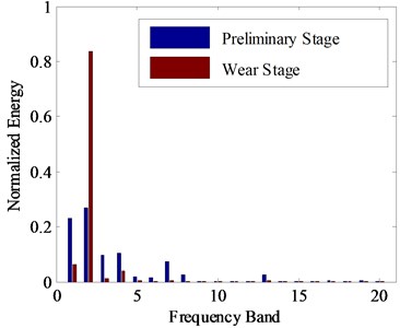
Fig. 8Comparison for different trend

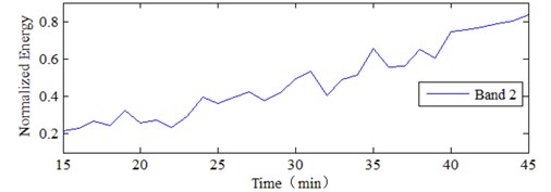
a) Energy trend

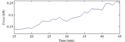
b) Force trend

Fig. 9Relationship for Band 2 energy and cutting force

3.1. Instantaneous reliability

Reliability is an important quality index of mechanical equipment, and the degree of reliability is one of the most important reliability evaluation indexes. The definition of reliability is that under prescribed conditions and within the limited time, the probability of equipment completes the required function without failure. However, in actual production the reliability based on probability statistics solution can’t help much. For analyzing and evaluating dynamic performance of the individual equipment, LU [2] firstly suggests the method to compute the reliability of equipment using interval integral defined by the failure threshold and index observation to predict the probability distribution of equipment performance degradation index. XU [16] uses the similar concept of reliability prediction and evaluation method and apply it in the instance estimation. If the instantaneous reliability of equipment at time $t$ is the probability which the device performance characteristics index $y_t$ is less than the failure threshold $y_c$:

In Eq. (8), $f_t\left(y_t\right)$ is the probability density function of the state characteristic $y_t$. As shown in Fig. 13, the red line is the failure threshold set, the probability which the state characteristic is greater than the failure threshold.

3.2. State space model

Estimation method is important for accurate analysis. The degradation process of equipment has the property of first order Markov. It means that the device status next time is only related to the device status this condition. The device status of different time is represented by $x_t$. The state characteristic extracted from monitored data is regarded as observed values, which is represented by $y_t$. Establishing equipment degradation SSM is as follows:

Eq. (9a) is the state equation, $A$ is the transformation matrix acting on the device status $x_t$. The future value of $x_t$ is only related to current condition, and is independent with the past status. It also named as Markov property. Eq. (9b) is the observation equation, and the mapping relationship between the system state and observation value is established. $C$ is the transformation matrix, $w_t$ is the process noise. Assuming the mean value is zero, the covariance for multivariate normal distribution is $w_t~N(0,Q)$. $e_t$ is the observation noise, and $e_t~N(0,R).$

Obviously, when the model parameters $\theta =\{A,C,Q,R\}$ and the device status $x_{t_0}$ are known, the mean value and variance of observed values $y_t$ at the moment $t>t_0$ can be directly calculated by Eq. (9). Setting the equipment failure threshold $y_c$, and the equipment reliability can be forecast by Eq. (8).

3.3. Solution of SSM

SSM solving method [17] is the Expectation Maximization (EM) algorithm, and its core is Kalman Filter. Kalman Filter is a recursive estimate, that is as long as the state estimation of last moment and the observation of current state are known, the estimate of current state can be calculated. If the system state vector $X$ is known, the optimal value of the parameter $\mathrm{}\theta =\{A,C,Q,R,{\mu }_0,{\epsilon }_0\}$ can be obtained through the Maximum Likelihood estimation (MLE). MLE method is by means of the maximizing likelihood function Eq. (11). According to the nature of the logarithmic function, when $P\left(Y\right|X,\theta )$ is a maximum value, the function $L\left(\theta \right)$ is also a maximum value. However, in fact state vector $X$ is unknown, the condition of parameter estimation is deficient:

The sequence of observations at $1~n$, $y_{1-n}$ is given, EM algorithm is estimating system parameters by Step Expectation and Maximization iterative. It can be expressed as:

3.4. Binary classification logistic regression model

Logistic research aims to find statistical principles between objective variables based on massive experiments and observations, which may be hidden in uncertain phenomenon. Logistic studies interrelation between variables by statistical model. For example, normal, failure, mild wear and severe wear in tool health monitoring research.

There are only two outputs in binary classification logistic regression model, output code zero and output code zero, which present the only two independent results, $t=\mathrm{1,2},\dots ,n$ is time coordinate of things. Element of parameter vector $X\left(t\right)=\{1,x_1\left(t\right),x_2\left(t\right),\dots ,x_m\left(t\right)\}$ at time $t$ is called covariant of $X\left(t\right)$, which influences occurrence of events, $m$ is the number of covariant. The conditional probability of the occurrence of $y_t$ can be expressed as:

where ${\beta }_0$, ${\beta }_1$, ${\beta }_2$,…, ${\beta }_m$ are model coefficients.

Assuming that there are two stages at time t, $y_t$ equals to 1 means normal stage, $y_t$ equals to 0 means failure stage. Expect the first element of covariant $X\left(t\right)$, other elements are different characteristic parameters at time $t$. Obviously, there is a kind of relation between device stage $y_t$ and $X\left(t\right)$, it should be nonlinear according to the features of rotating components.

Suppose stage monitoring characteristic vector is $\left(t\right)$, the ratio between the reliability function $R\left(t\right|X\left(t\right))$ of rotating component and the cumulative failure distribution function $F\left(t|X\left(t\right)\right)=1-R\left(t\right|X\left(t\right))$ satisfies the following equation:

Model coefficients ${\beta }_0$, ${\beta }_1$, ${\beta }_2$,…, ${\beta }_m$ reflect the change of odds ratio, if ${\beta }_i$ is bigger than zero, the possibility goes up with the increase of $x_i$, otherwise, the opposite. If ${\beta }_i$ equals to zero, it doesn’t work in this model. After the estimation of ${\beta }_0$, ${\beta }_1$, ${\beta }_2$,…, ${\beta }_m$, the reliability function $R\left(t\right|X\left(t\right))$ can be expressed as:

The confidence interval of 90 % is:

In this equation $\beta =\{{\beta }_0,{\beta }_1,{\beta }_2,\dots ,{\beta }_m\}$, $var$ denotes variance:

where $Cov\left(\beta \right)X\left(t\right)$ denotes covariance matrix of coefficients

3.5. Flow chart for reliability estimation

In this paper, Wavelet packet feature extraction and SSM method are applied to the reliability evaluation of rotating machine working condition. Firstly, signals about machine working conditions are collected based on-line monitoring technology for equipment. Secondly, wavelet packet energy is applied on characteristic extraction for the monitored signals. Frequency band energy is determined to be as characteristic parameter. Then, the degradation characteristics of signal to noise ratio is improved by moving average filtering processing. In the end, SSM is established to predict. The parameters will update based on different working condition data. It is more suitable for practical problem solution, which can be satisfied with prognostics. MC working condition degradation process is used to verify the effectiveness of the method in this research.

4.1. Experiment data analysis

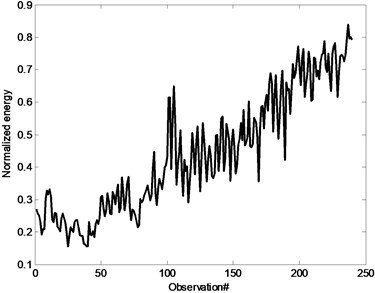
To verify the effectiveness of the proposed method, a wearing experiment is carried on for MC. It is an accelerated experiment. The monitored data process can be similarly determined as shown in Fig. 4. To demonstrate the degradation process for MC wearing process, wavelet packet is used for decomposition and normalization energy are used to determine the characteristic parameter to estimate the wearing process. Based on the above investigation, the second frequency band is used for feature extraction and reliability estimation. The wearing process for MC based on different time is shown as Fig. 10. Obviously, the developing trend is the same with wearing time for this accelerated experiment. It can also demonstrate that the second frequency band can be used to estimate the wearing process. But it is obvious there is data fluctuation as noise interference for monitored process.

Fig. 10The degradation process for MC based on the second frequency band energy normalization

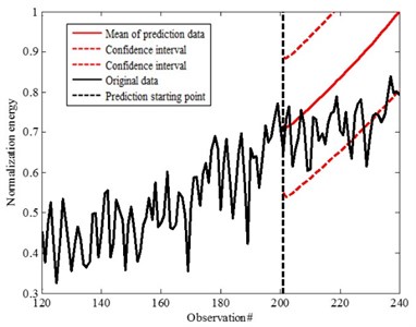
The prediction analysis based on the 150th and 200th points acquisition data are carried on, shown as Fig. 11 and Fig. 12 based on SSM. For the 150th point, the mean value based on the prediction deviates from the degradation trend. The confidence interval can't reflect the prediction accuracy. Although the mean value is not the same with the degradation process for 200th point prediction, it is almost same with the degradation process. There is also difference for the confidence interval. It is obviously the analysis result is not good for the prediction. It is important to improve the prediction accuracy. It also means that SSM depends on the degradation process. The result has been greatly influenced by the data fluctuation shown as Fig. 11 and Fig. 12. Prediction accuracy is influenced as the data fluctuation. Therefore, it is important to process the data for accurate analysis. To improve the prediction accuracy, moving average is carried on for the analysis.

Fig. 11Prediction data for the 150th step

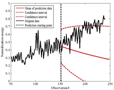
Fig. 12Prediction data for the 200th step

4.2. Moving average

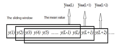
Moving averageis a data pre-processing method with smoothing and filtering effect. It can filter out the frequent stochastic fluctuant data [18]. At the same time, it can also conclude the changing process of random error. Thus, the statistical characteristics can be estimated. As shown in Fig. 13, let the length $L$ sliding window move through the sequence $\{y\left(t\right),t=\mathrm{1,2},\dots ,N\}$. Then, compute the mathematic average for all elements inside the window and put the average value as one element of the new sequence, and the new sequence is moving average of $y\left(t\right)$. Mathematical expression is as follows:

Fig. 13The moving average method

Based on the moving average process, taking 50 observed values for average. Fig. 14 presents the comparison for original one and after moving average. It is obvious that the degradation data trend is almost linear after moving average. It can effectively reduce the data fluctuation for the effect of prediction. It is good to improve the accuracy for prediction. As it is almost linear, Kalman filter is better for the SSM prediction. Initial parameters setting is as following for the SSM prediction:

Fig. 14Comparison for original data and after moving average

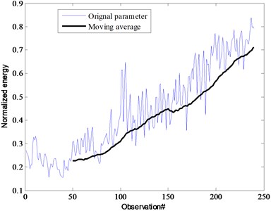
Fig. 15 and Fig. 16 are the prediction results of SSM established by observed values of two different time steps 150th and 200th point based on different confidence 90 % and 95 %. The mean of prediction for the 200th point is almost the same with original data (characteristic parameters after moving average) which is within the confidence interval. In this research, the confidence is defined as 90 %. It is better compared with 150th point prediction. It is also obvious that the prediction accuracy can be improved with time step increment based on comparison for different working conditions. But it is much better compared with Fig. 11 and Fig. 12 for the data without moving average. That also means it could effectively improve the accuracy with moving average. Data preprocessing is important to assure the accuracy prediction. By using moving average, the fluctuation from the characteristic parameters can be effectively removed. It is also helpful to improve the prediction accuracy. As well, confidence also has effect on the analysis. Based on the prediction, the development is within the confidence.

Fig. 17 is the reliability prediction results of the corresponding MC. The actual life of cutter is 236. Set the reliability threshold $R=$ 0.5. The prediction nonfatal failure moment distribution of cutter is 229 and 235, which is consistent with the actual situation. It is better for 150th though it is a little far from the failure point. But it can also present accurate prediction result. It is much better for 200th prediction compared with 150th. As well, it can significantly reduce the prediction error and improve the prediction accuracy. Based on the parameters updated for every step prediction, it can be obtained that the prediction will get more and more accurate with parameters update. Therefore, this method is effectively verified to the analysis of practical problems. It can be used on the prediction and reliability analysis for MC wearing condition as this is real working machine.

Fig. 15Prediction data of 90 % confidence

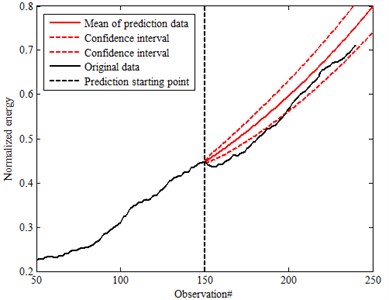
a) The 150th prediction for moving average data

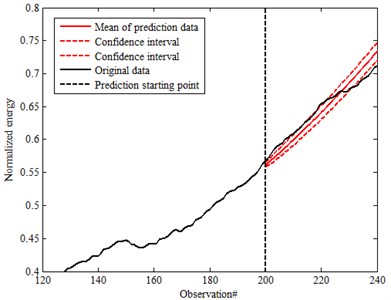
b) The 200th prediction for moving average data

Fig. 16Prediction data of 95 % confidence

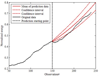
a) The 150th prediction for moving average data

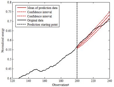
b) The 200th prediction for moving average data

Fig. 17The reliability prediction results at different time

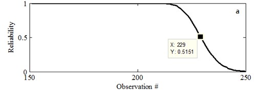
a) Prediction based on 150#

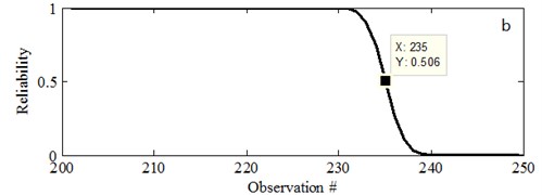
b) Prediction based on 200#

4.3. Discussions

Based on above analysis, it is clear the SSM has good performance on prediction analysis as it is based on EM process. It is an iteration process which is just based on the current data for prediction. Therefore, it is good for reliability analysis. At the same time, the prediction result is also influenced by the data fluctuation if there is not moving average process. It also demonstrates the degradation trend which is very important for the prediction and reliability analysis. How to effectively determine the best suitable parameters for condition reliability analysis is the basis.

AE signal is good to demonstrate the wearing process for MC and failure process. It is good for moving average process to reduce fluctuation effect for SSM analysis based on the feature extraction. Actually, only a parameter is used in this investigation to verify the effectiveness of SSM model on prediction. Condition monitoring is the dispersive for different data. At the same time, it needs more information to estimate machine working conditions and reliability analysis. It is better to use much data analysis for reliability analysis. But it depends on the monitoring process and the degradation process for different parameters. The monitored data can be integrated together for better demonstration of machine condition parameters. Then, a parameter is used for reliability analysis. Otherwise, more monitored parameters can be input in Eq. (9). The prediction process can be carried on for analysis. As the degradation process is not linear for more parameters prediction, improved Kalman filter can be used for analysis.