Numerical optimization of vehicle noises in multi-peak frequency points based on hybrid genetic algorithm and simulated annealing

Qu, Xiao-jun; Liang, Hai-long; Zhang, Bo-chao; Cui, Xu-yang

doi:10.21595/jve.2016.16669

Journal of Vibroengineering

Browse Journal

Submit article

Published: 30 June 2016

Check for updates

Numerical optimization of vehicle noises in multi-peak frequency points based on hybrid genetic algorithm and simulated annealing

Xiao-jun Qu¹

Hai-long Liang²

Bo-chao Zhang³

Xu-yang Cui⁴

^{1, 2, 3}North University of China (Shuozhou), Shuozhou, China

⁴School of Mechanical Engineering, Tianjin University, Tianjin, China

Corresponding Author:

Bo-chao Zhang

Cite the article Download PDF

Downloads 1416

WoS Core Citations 1

CrossRef Citations 1

Abstract

The finite element model of Body in White was built, and the corresponding modes were computed in this paper. These computational modes were then compared with experimental results. The small errors showed that the accuracy of the finite element model can satisfy the computational requirements. Based on the verified finite element model, acoustic cavities in the vehicle were extracted to build a boundary element model. Sound pressure levels at all passengers in the vehicle were then computed, compared and analyzed. Results indicated that the sound pressure curve had 6 peak noises. Using the characteristic frequency weight coefficient and field point weight coefficient, the body panels which made large acoustic contributions to the comprehensive sound field under multi-characteristic frequencies were determined. Finally, the improved genetic algorithm based on simulated annealing was used to optimize the key body panels, and peak noises at researched field points after the optimization were further computed. The computational results were compared with those of the original structure, which presented that the noise was improved at most frequency points in the spectrum and peak noises were suppressed obviously.

1. Introduction

With the rapid development of light-weight technologies, the dynamic performance of the vehicle has been improved obviously. However, vibrations and noises in the low frequency have also been increased [1]. Loudness of noises in the low frequency was not very large, but long-term noises can very easily cause discomfort and driving safety [2]. Currently, researches on noises in the low frequency have obtained a lot of achievements. Citarella [3] applied the boundary element method to research acoustic responses and panel contributions, and found the panels which had large influences on driver’s noises. However, the research was not verified by the corresponding experiment, and measures were not adopted to improve noises. Sung [4] applied the finite element method to analyze noises in the vehicle and considered the coupling between body structures and sound field, finding that the coupling had serious influences on sound field. Langley [5] applied the boundary element method to predict sound radiation in the structure, but the adopted vibration excitation was only the unit harmonic force and did not satisfy actual situations. Chen [6] researched the instant values of sound pressures in 20 Hz~250 Hz based on the same road surface and different speeds, but effective values of sound pressures in the analyzed frequency band were not computed. Ding [7] applied the dynamic substructure method based on vibro-acoustic coupling to research the quantitative relations between noises and parameters of a suspension. Mohanty [8] applied the finite element method and the boundary element method to analyze the sound field of a truck, and computed the structural vibration response, finding that the noise in the vehicle was improved by adding sound absorption materials.

However, the mentioned researches mainly focused on panel contributions to a single response peak. As for a characteristic field point with multiple peak noises, the panel always had different contributions and characteristics to the different peaks, so that its improvement can hardly be determined. Meanwhile, a single field point cannot completely reflect acoustic characteristics of the full sound field, while the improvement of noises at one field point may cause deterioration of noises at other field points. Han [9, 10] proposed that the weighted summarization could be used to compute panel contributions to full acoustic characteristics in the vehicle and obtained outstanding noise reduction effects using the damping technology, but he had not adopted any optimization algorithm to conduct on an optimization analysis. Panel contributions based on acoustic transfer vector method were conducted in this paper. Then, the characteristic frequency weight coefficient and field point weight coefficient which can be used to determine the key panels were proposed. Finally, the improved genetic algorithm was used to optimize the sound field.

2. Theories of acoustic transfer vector

As the natural characteristics of a system, the acoustic transfer vector was a linear relation between the vibration velocity in the structural surface and sound pressures. When the pressure disturbance was very small, the acoustic equation can be considered as linear. A linear relation can be built between the input and output. In this way, the sound pressure at one point of the sound filed can be obtained as follows [11]:

1

p = {\{A T V (ω)\}}^{T} \{υ_{n} (ω)\},

where: $\{A T V\}$ was the acoustic transfer vector, $υ_{n}$ was the vibration velocity in the structural surface, $ω$ was an angle frequency.

A linear relation between the vibration velocity and the sound pressure can be built using ATV. The physical significance of ATV can be understood as the sound pressure which was caused by the unit vibration velocity. ATV was related to the following physical parameters: geometric shape of the structure, processing of the structural surface, field point positions, computational frequencies and physical parameters of an acoustic medium.

In equation (1), $υ_{n}$ can be obtained by projecting the structural displacement vector on the normal of the structural surface, as follows:

2

\{υ_{n}\} = j ω Ω_{n} \{M R S P (ω)\},

$Ω_{n}$ was a vector matrix of structural modes. $\{M R S P (ω)\}$ was a vector which was composed of mode participant factors. Therefore, the sound pressure at any point in the sound field can be obtained as follows:

3

p = {\{A T V (ω)\}}^{T} j ω Ω_{n} \{M R S P (ω)\} .

3. The coupling model between vibrations and acoustics

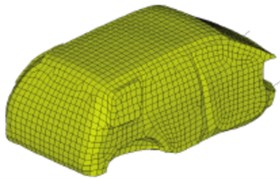
3.1. The finite element model

The analyzed body in this paper was composed of some panels. 4-node or 3-node shell elements were used for modeling. Triangular elements occupied 7.8 % of the total elements. ACM2 model was used to simulate the point welding. RBE2 was used to simulate the bolt connection. The finite element model of Body in White was built in the HYPERMESH, as shown in Fig. 1. The generation of the model occupied 2/3 of the analyzed time and played a key role in deciding whether CAE technology was reliable. Accuracy of the model could directly decide the computational time and accuracy. During modeling, non-bearing structures such as wing panels and bumpers which only had very small influences on structural deformation and mechanical performance were ignored. Technological structures such as assembly holes, steps and round angles which only had very small influences on the structural performances were deleted. Additionally, through mode experiments and CAE technology, the natural frequencies of first 4 orders were compared and taken as the judgment standards. Parameters were modified and set for the finite element model, so that they could reach the optimal. It was shown in Table 1 that the relative errors between experiment and simulation were small. Obviously, the finite element model in this paper had high accuracy and can be used as the model for the further analysis. The mode was shown in Fig. 1.

Fig. 1The finite element model of body in white

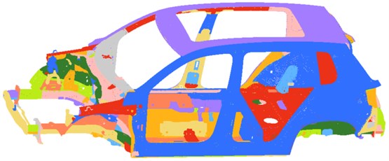
Table 1Comparisons between experiment and simulation

Order	Simulation value / Hz	Experiment value / Hz	Mode	Relative Error / %
1	30.8	31.31	Top dislocation	–1.62
2	38.0	36.67	First-order torsion	3.62
3	40.0	38.41	First-order bending	4.14
4	42.9	44.29	Horizontal sway of front cabin	–3.14

Fig. 2Modes of body in white at first 4 orders

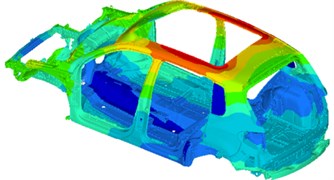
a) 30.8 Hz

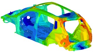
b) 8.0 Hz

c) 40.0 Hz

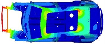
d) 42.9Hz

3.2. The boundary element model

The boundary element model can be used to compute the sound field of the enclosed cavity and the opened cavity. The boundary element model required shell elements. During computing the sound field in the vehicle, it was generally processed as an enclosed cavity. When the fluid simulation was conducted in Virtual.Lab, behaviors such as reflection, diffraction and refraction of sounds were taken into account. Therefore, errors of the computational results mainly come from inaccuracy of material definitions, insufficient model and boundary conditions. In order to ensure that the largest size of an acoustic element was smaller than 1/6 of the shortest wavelength of the computational frequency, the element length was set to be 60 mm-70 mm. Acoustic meshes shall be basically consistent. The computational accuracy of a fluid model was controlled by most elements, so the size of elements should be uniform. The partial fine meshes cannot increase the computational accuracy. However, meshes can be divided appropriately in a more refined form at these places where the structure model was coupled with the fluid model.

In this paper, the boundary element model was built with the following steps: Firstly, the finite element meshes were enclosed; cavity meshes in the vehicle were extracted; Face command was then used to extract meshes on cavity boundaries; and the simplified seat meshes were also added into the model.

Fig. 3Boundary element model of the vehicle

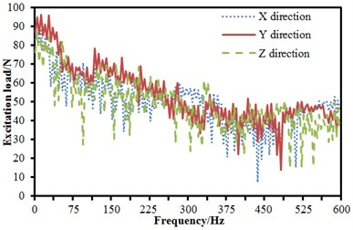
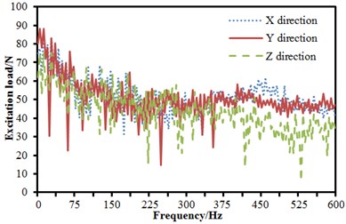
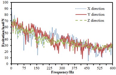
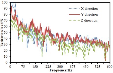
Through the experiment, forces which were loaded by the engine onto 4 suspension points were shown in Fig. 4. The excitation force was applied at corresponding positions of the finite element model in Fig. 1. Then, the model was input into Virtual.Lab and coupled with the boundary element model in Fig. 3. Vibration characteristics of the structure were mapped into the boundary element model. In this way, the boundary element meshes can obtain all characteristics of the structural model and realize the vibro-acoustic coupling. 4 field points were set in the boundary element model and stood for driver, co-driver, left passenger and right passenger. Sound pressures at all passengers could be observed. Results were presented in Fig. 5. It was shown in Fig. 5 that sound pressure levels basically had the same tendencies at 4 field points, where 6 sound pressure peaks were presented, and the corresponding frequencies were 51 Hz, 110 Hz, 245 Hz, 262 Hz, 330 Hz and 382 Hz, respectively. The maximum value of sound pressure levels was more than 85 dB, but the minimum value was only 50 dB. Their difference approached 40 dB, and serious roar sound would be presented in the vehicle. Therefore, it was necessary to take some measures to reduce 6 peak noises.

In order to verify the effectiveness of the computational model, noises were tested in a semi-anechoic chamber, as shown in Fig. 6. The experimental environment had very large influences on the results. The semi-anechoic chamber as an acoustic lab was used to simulate a semi-free sound field. In the space, there were only direct sounds and primary reflection sounds. The experimental method was shown as follows: in the semi-anechoic chamber, the vehicle stably ran under an idling condition, while sound pressures of driver, co-driver, left passenger and right passenger were tested and recorded. During the experiment, sound pressure signals were collected by a piezoelectric microphone [12, 13]. The experimental system was LMS Test.Lab. Sampling frequency was 25600 Hz and the resolution ratio was 2 Hz. After completing collection, time-domain signals were processed by spectral analysis and compared with computational results. With sound pressures of the driver as an example, results were shown in Fig. 7.

It was shown in Fig. 7 that the consistency was good, but there were some errors between simulation and experiment mainly because that the boundary conditions of the computational model could hardly be kept consistent with actual situations.

Fig. 4Excitation forces of 4 points on the body

a) Point 1

b) Point 2

c) Point 3

d) Point 4

Fig. 5Sound pressure levels at all passengers in the vehicle

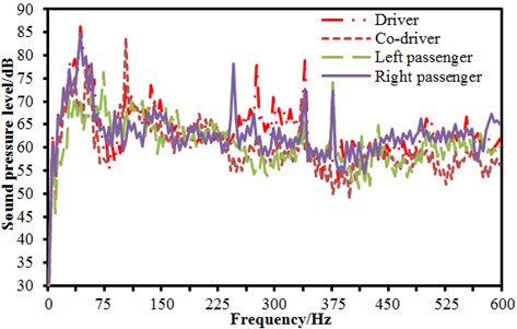
Fig. 6The experimental noise in the vehicle

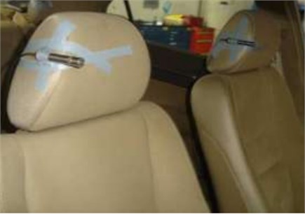
Fig. 7Comparison of noises between experiment and simulation

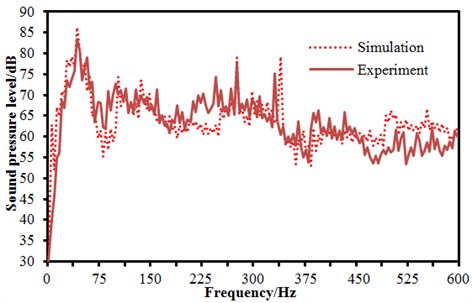
Fig. 8Contribution color bar of panels in field points

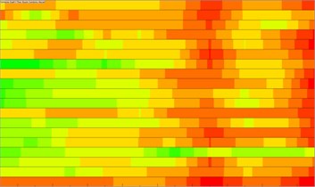
a) Driver

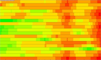
b) Co-driverr

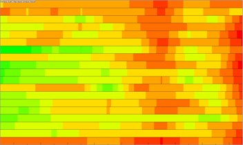
c) Left passenger

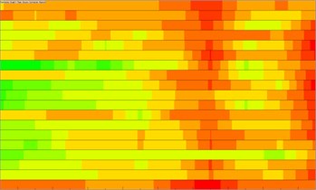
d) Right passenger

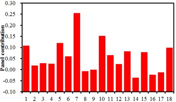
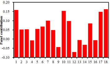
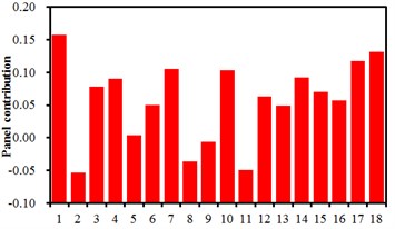
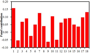
Noises were always caused by vibrations of body panels. Therefore, in order to reduce noises in the vehicle, it was necessary to adopt some measures to reduce radiation noises of panels. ATV method mentioned in Section 2 can effectively recognize the panels which made large contributions to noises. Therefore, noises can be effectively improved by taking some measures to these panels. Firstly, acoustic cavity panels were grouped according to functions and characteristics of each panel, as shown in Table 2. Based on the vibro-acoustic coupling model, the panel contribution was conducted. Contributions made by panels at each field point were shown in Fig. 8. Contributions made by panels at each frequency point could be obtained through further normalization of these contributions, and results were presented in Fig. 9. It was shown in Fig. 9 that panel contributions at 6 peak frequency points were not completely consistent. As can be seen from this figure, it was also difficult to recognize the panels which made large contributions to peak noises. Therefore, it was necessary to adopt methods based on the information to recognize the panels which had large influences on noises of multi-characteristic frequency points.

Table 2ID of acoustic cavity panels

Panel ID	Panel	Panel ID	Panel
1	Firewall	10	Top panel
2	Front floor	11	Left front door
3	Middle floor	12	Right front door
4	Rear floor	13	Left rear door
5	Left rear wheel hood	14	Right rear door
6	Right rear wheel hood	15	Front wind shield
7	Back door inner panel	16	Left side
8	Rear wind shield	17	Right Side
9	Skylight glass	18	Dash panel

Fig. 9Panel contributions at 6 peak frequency points

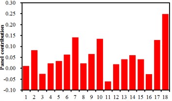
a) 51 Hz

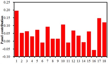
b) 110Hz

a) 51Hz

b) 110Hz

e) 330Hz

f) 382Hz

4. Acoustic contributions of multi-characteristic frequencies

Based on the mentioned analysis, different acoustic contributions were made by body panels to field points under different characteristic frequencies. However, the importance of field points and characteristic frequencies in the comprehensive sound field in the vehicle can be relied on, and different weight can be given to every filed point and every response characteristic frequency. An expression of the acoustic contribution was proposed in the paper.

4

{(P_{c})}_{T o t a l} = \sum_{N = 1}^{m} (β_{N} \sum_{i = 1}^{n} α_{i} ∙ {(P_{c})}_{i, N}),

wherein, ${(P_{c})}_{T o t a l}$ was the total contribution of all panels to the comprehensive sound field under multi-characteristic frequencies; ${(P_{c})}_{i, N}$ was the acoustic contribution of all divided panels at a characteristic frequency $i$ of a field point $N$ ; $n$ was the number of characteristic frequencies related to the contribution analysis of panels; $α_{i}$ was the weight coefficient of each characteristic frequency, which was used to distinguish different importance degrees of characteristic frequencies; and $β_{N}$ was the weight coefficient of the $N$ th field point, which was determined by the importance of this field point in the sound field. This weight coefficient can be determined by the ratio of the sound pressure response at main characteristic frequency of the field point $N$ occupied in the total sound pressure response of all field points, and $β_{N}$ can be expressed as follows:

5

β_{N} = \frac{\sum_{i = 1}^{n} D_{N, i}}{\sum_{i = 1}^{n} D_{1, i} + \sum_{i = 1}^{n} D_{2, i} + \dots + \sum_{i = 1}^{n} D_{m, i}} = \frac{\sum_{i = 1}^{n} D_{N, i}}{\sum_{N = 1}^{m} \sum_{i = 1}^{n} D_{N, i}},

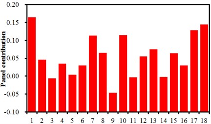
wherein, $D_{N, I}$ was the sound pressure response of the field point $N$ at the characteristic frequency $i$ . The influence of panels on the acoustic characteristics of the sound field could be fully characterized by the comprehensive sound field contribution under multi characteristic frequencies in Eq. (4). Its magnitude was applied to represent this panel contribution to the comprehensive acoustic characteristics. Combined with the studied vehicle, the panel area was 18, $n$ = 6, $m$ = 4; the same degree of attention was paid to every characteristic frequency, $α_{i}$ =1; in line with Eq. (5), the weights of all field points could be computed and obtained as Table 3. The comprehensive acoustic contributions of panels were ranked as Fig.10. It was shown in the figure that panels with ID of 1, 7, 10, 17 and 18 had large influences on 6 peak noises, and the corresponding panels were firewall, back door inner panel, top panel, right side and dash panel, respectively. Therefore, 6 peak noises can be effectively reduced through applying noise reduction measures to these panels, so that the environment can be improved.

Table 3Weight coefficient βN of each field point

Field point	Driver	Co-driver	Left passenger	Right passenger
$β_{N}$	0.35	0.26	0.21	0.18

Fig. 10Panel contribution of the sound field under multi-featured frequencies

5. Numerical optimization of noises based on the improved genetic algorithm

Through ATV analysis, panels which had serious influences on 6 peak noises in the vehicle have been recognized. Optimization design of these panels was conducted. As a result, their vibration characteristics can be reduced, and radiation noises can be improved.

5.1. Analysis of optimization problems

In the boundary element model, the interior parts were taken into account, and each panel was covered by a layer of damping structure. Therefore, the optimization mainly considered thicknesses of panels and damping materials to improve vibration effects. Stiffness of a panel mainly depended on the first order frequency. Therefore, during optimization design, it was necessary to ensure that the frequency of the optimized panel was more than that of the original structure. In addition, the mass of the optimized panel should not be higher than 50 % of mass of the original structure. Vibration velocities of 5 key panels needed to be optimized, so that it was a multi-objective optimization problem [14-17].

6

\min f (x) = \min \{υ_{1} (a), υ_{2} (b), υ_{3} (c), υ_{4} (d), υ_{5} (e)\},

a = \{a_{1}, a_{2}\}, b = \{b_{1}, b_{2}\}, c = \{c_{1}, c_{2}\}, d = \{d_{1}, d_{2}\}, e = \{e_{1}, e_{2}\},

ω_{1} \geq 39.1, ω_{2} \geq 26.3, ω_{3} \geq 27.4, ω_{4} \geq 36.1, ω_{5} \geq 41.2,

m_{1} \leq 17.5, m_{2} \leq 12.7, m_{3} \leq 13.9, m_{4} \leq 16.2, m_{5} \leq 10.5,

0 \leq a_{i} \leq 1, 0 \leq b_{i} \leq 1, 0 \leq c_{i} \leq 1, 0 \leq d_{i} \leq 1, 0 \leq e_{i} \leq 1,

i \in (1,2) .

5.2. Selection of optimization algorithm

The paper tried to use the genetic algorithm [18-21] to research this optimization problem. Its necessity was mainly presented as follows.

The genetic algorithm has been widely applied in the multi-objective optimization problem. It was a relatively mature optimization algorithm, and the operations were relatively convenient.

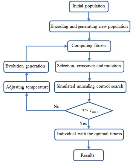
Genetic Algorithm (GA) was a self-adaptive global search algorithm which was formed based on generation and evolution in a natural environment [22, 23]. GA was mainly conducted by operating chromosomes, and it was not directly related with parameters and did not depend on the gradient information. Only a fitness function was applied as an evaluation criterion, and knowledge in other special fields was not required. Random regulations, rather than determined regulations, were used for searching. No special requirement was proposed for the searched space, and derivation was not required. The algorithm had the advantages of simple operation and quick convergence. It was especially applicable to complex and non-linear problems which can hardly be solved by traditional search algorithms. However, the traditional genetic algorithm had two serious defects: premature convergence can take place very easily, and search efficiency was low at later evolution stage. As a result, the result obtained by the final search was always the locally optimal solution rather than the globally optimal solution. The traditional genetic algorithm cannot effectively overcome the premature convergence, so that a lot of current researches focused on finding how to improve the traditional genetic evolution idea. SA algorithm had a simple computation process, strong robustness and good optimization capacity, but performance of the algorithm depended on initial values and was highly sensitive to parameters, while the capability of globally search of optimal solutions was bad. Based on this, we can find that two algorithms were highly complementary. Firstly, SA algorithm made GA select search space in a more suitable direction and can avoid local optimization. Secondly, GA can provide new solutions for SA operators during crossover and mutation. Finally, solutions obtained by SA operators can selectively provide GA with new groups to improve convergence speed of GA. In this way, the hybrid algorithm can obtain the globally optimal solution in a short term. Optimization processes with the improved genetic algorithm based on SA were shown in Fig. 11.

In addition, the commercial software ISIGHT was used in the optimization in the paper. Modules of genetic algorithm and simulated annealing algorithm were integrated in the software. Through an intermediate program, the simulated annealing algorithm can be integrated into the genetic algorithm. It was unnecessary to separately program a complex program. In this way, time was saved, the computational efficiency was increased, and cost was also reduced.

Fig. 11Flow diagram of the improved genetic algorithm

During the optimization, the initial size of the population was set to 45, the crossover rate was 0.95, and the mutation rate was 0.05. As an important parameter in the optimization design process, the fitness reflected the convergence speed of the genetic algorithm. The fitness was changed with the evolutionary generation number. It can be obtained that the fitness value was gradually stabilized when the evolution generation was 75. However, the fitness value in the traditional genetic algorithm was generally stabilized and the result was converged after 240 generations. Therefore, it was presented that the improved genetic algorithm had obvious advantages in the multi-objective optimization.

5.3. Analysis of the optimized result

Based on the mentioned optimization, the thickness of each penal can be obtained. The optimized panels were applied in the vehicle to compute sound pressure levels at 4 field points.

A comprehensive indicator was introduced to express the differences before and after optimization because it was aimed at observing the improved effect of multiple field points:

7

P_{s y n} (ω) = \sqrt{\sum_{N = 1}^{m} P_{N} {(ω)}^{2}},

wherein: $P_{s y n}$ was the comprehensive noise indicator of multiple field points in the vehicle, and $P_{N} (ω)$ was the noise spectrum of field point $N$ .

Comparisons of the interior noise before and after optimization were shown in Fig. 12. As can be seen from the results, the noise has been reduced obviously. In addition, the total noises at 6 characteristic frequencies before and after optimization were listed in Table 4. SPLs of each field point were further presented in Fig. 13, and they were obviously improved. Therefore, the optimization method proposed in the paper was effective.

Fig. 12Comparisons of spectrum noises before and after optimization

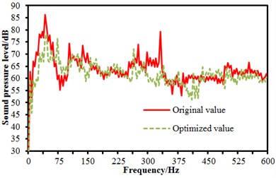
a) Driver

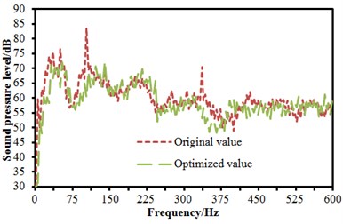
b) Co-driver

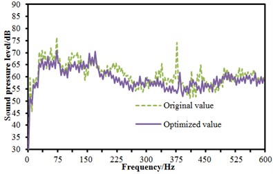
c) Left passenger

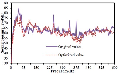
d) Right passenger

Fig. 13Comparisons of average noises before and after optimization

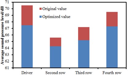
Table 4Noises at 6 characteristic frequencies before and after optimization

Frequency	Before optimization	After optimization	Change
51 Hz	86.3 dB	78.5 dB	–7.8 dB
110 Hz	84.8 dB	73.6 dB	–11.2 dB
245 Hz	79.4 dB	72.3 dB	–7.1 dB
262 Hz	78.4 dB	70.3 dB	–8.1 dB
330 Hz	80.2 dB	68.5 dB	–11.7 dB
382 Hz	75.1 dB	65.2 dB	–9.9 dB

6. Conclusions

The finite element model of Body in White was built, and the corresponding modes were computed in this paper. These computational modes were then compared with experimental results. The small errors showed that the accuracy of the finite element model can satisfy the computational requirements. Based on the verified finite element model, acoustic cavities in the vehicle were extracted to build a boundary element model. Sound pressure levels at all passengers in the vehicle were then computed, compared and analyzed. Results indicated that the sound pressure curve had 6 peak noises. Using the characteristic frequency weight coefficient and field point weight coefficient, the body panels which made large acoustic contributions to the comprehensive sound field under multi-characteristic frequencies were determined.

Genetic Algorithm (GA) was a self-adaptive global search algorithm which was formed based on generation and evolution in a natural environment. This algorithm was outstanding in global search capability but insufficient in the local search capability. Simulated annealing (SA) was an algorithm featured with the outstanding local search ability and widely used in combinational optimization problems. As a result, they were combined to present their mutual advantages and use the global search capability of GA and local search capability of SA. The improved GA was used to optimize this problem in this paper.

Finally, the optimal combination of panel and damping material was determined. It was shown from the computational results of the optimized proposal that the interior noise was improved obviously. Therefore, the panel optimization based on the comprehensive sound field proposed in the paper was effective, which also provided a more complete and systematic optimization method for the vibration noise reduction of body panels.

References

Zhu C. C., Qin D. T., Li R. F. Study on coupling between body structure dynamic and interior noise. Chinese Journal of Mechanical Engineering, Vol. 38, Issue 8, 2002, p. 54-58.

Publisher
Yang B., Zhu P., Yu H. D., et al. Auto-body NVH structure sensitivity analysis based on modal analysis method. China Mechanical Engineering, Vol. 19, Issue 3, 2008, p. 361-364.

Search CrossRef
Citarella R., Federico L., Cicatiello A. Modal acoustic transfer vector approach in a FEM-BEM vibro-acoustic analysis. Engineering Analysis with Boundary Elements, Vol. 31, Issue 3, 2007, p. 248-258.

Publisher
Sung S. H., Nefske D. J. A coupled structural-acoustic finite element model for vehicle interior noise analysis. Transactions of the ASME on Vibration, Acoustic, Stress, and Reliability in Design, Vol. 106, 1984, p. 314-318.

Publisher
Langley R. S. A dynamic stiffness/boundary element method for prediction of interior noise levels. Sound and Vibration, Vol. 163, Issue 2, 1993, p. 207-230.

Publisher
Chen C. M., Sun W. Numerical simulation and analysis of cab interior noise with the consideration of road surface roughness. Journal of Vibration and Shock, Vol. 27, Issue 8, 2008, p. 102-105.

Search CrossRef
Ding W. P. Quantitative relationship between low frequency interior noise and suspension characteristic parameter of a vehicle. Noise and Vibration Control, Vol. 5, 2006, p. 70-73.

Search CrossRef
Mohanty A. R., Pierre B. D. Structure-borne noise reduction in a truck cab interior using numerical techniques. Applied Acoustics, Vol. 59, 2000, p. 1-17.

Publisher
Han X., Yu H. D., Guo Y. J. Study on automotive interior sound field refinement based on panel acoustic contribution analysis. Journal of Shanghai Jiaotong University, Vol. 42, Issue 8, 2008, p. 1254-1258.

Search CrossRef
Han X., Guo Y. J., Yu H. D. Interior sound field refinement of a passenger car using modified panel acoustic contribution analysis. International Journal of Automotive Technology, Vol. 10, Issue 1, 2009, p. 79-85.

Publisher
Wang E. B., Zhou H., Xu G. Acoustic-vibration optimization based on panel acoustic contribution analysis of vehicle body. Journal of Jiangsu University (Natural Science Edition), Vol. 33, Issue 1, 2012, p. 25-29.

Search CrossRef
Li J. Q., He S. Q., And Ming Z. An intelligent wireless sensor networks system with multiple servers communication. International Journal of Distributed Sensor Networks, Vol. 7, 2015, p. 1-9.

Publisher
Wong K. W., Lin Q., Chen J. Error detection in arithmetic coding with artificial markers. Computers and Mathematics with Applications, Vol. 62, Issue 1, 2011, p. 359-366.

Publisher
Zhu Z., Xiao J., Li J. Q., et al. Global path planning of wheeled robots using multi-objective memetic algorithms. Integrated Computer-Aided Engineering, Vol. 22, Issue 4, 2015, p. 387-404.

Publisher
Liang Zhengping, Song Ruizhen A double-module immune algorithm for multi-objective optimization problems. Applied Soft Computing, Vol. 35, 2015, p. 161-174.

Publisher
Chen J., Lin Q., Shen L. L. An immune-inspired evolution strategy for constrained optimization problems. International Journal on Artificial Intelligence Tools, Vol. 20, Issue 3, 2011, p. 549-561.

Publisher
Chen J. Y., Lin Q. Z., Hu Q. B. Application of novel clonal algorithm in multiobjective optimization. International Journal of Information Technology and Decision Making, Vol. 9, Issue 2, 2010, p. 239-266.

Publisher
Mühlenbein H., Schomisch M., Born J. The parallel genetic algorithm as function optimizer. Parallel Computing, Vol. 17, Issue 6, 1991, p. 619-632.

Publisher
Juang C. F. A hybrid of genetic algorithm and particle swarm optimization for recurrent network design. IEEE Transactions on Systems, Man, and Cybernetics, Part B: Cybernetics, Vol. 34, Issue 2, 2004, p. 997-1006.

Publisher
Baker B. M., Ayechew M. A. A genetic algorithm for the vehicle routing problem. Computers and Operations Research, Vol. 30, Issue 5, 2003, p. 787-800.

Publisher
Hartmann S. A self-adapting genetic algorithm for project scheduling under resource constraints. Naval Research Logistics (NRL), Vol. 49, Issue 5, 2002, p. 433-448.

Publisher
Lin Q., Wong K. W., Chen J. An enhanced variable-length arithmetic coding and encryption scheme using chaotic maps. Journal of Systems and Software, Vol. 86, Issue 5, 2013, p. 1384-1389.

Publisher
Du Z. H., Zhu Y. Y., Liu W. X. Combining quantum-behaved PSO and K2 algorithm for enhance gene network construction. Current Bioinformatics, Vol. 8, Issue 1, 2013, p. 133-137.

Publisher

Cited by

Vehicle Interior Noise Prediction Based on Elman Neural Network

(2021)

About this article

Received

24 November 2015

Accepted

16 June 2016

Published

30 June 2016

SUBJECTS

Acoustics, noise control and engineering applications

DOI

https://doi.org/10.21595/jve.2016.16669

Keywords

panel contribution

acoustic transfer vector

improved genetic algorithm

multi-characteristic frequencies

Acknowledgements

This work was supported by Heilongjiang Provincial Natural Science Foundation (No. F201422).

This is an open access article distributed under the Creative Commons Attribution License, which permits unrestricted use, distribution, and reproduction in any medium, provided the original work is properly cited.

Previous article in issue Previous Next article in issue Next

Research article

2017 12 31

A novel MPP-NSGA algorithm and its application in optimization for radiated noises in the aircraft cabin

Jie Li, Wei Xing Liu, Yu Zhu Zhang, Ling Zhang, Shan Shan Li

Research article

2017 09 30

Numerical optimization for vibration and noise of the wheel based on PSO-GA method

Yi Ji, Hai Jun Fu, Kun Hua Chen

Research article

2017 06 30

Numerical optimization of sound pressure responses for the dash panel based on automatically matched layer and genetic algorithm

Xin Zhe Zhang, Guo Jie Zhang

Research article

2016 03 31

The noise control of minicar body in white based on acoustic panel participation method

Yongliang Wang, Xunpeng Qin, Li Lu, Huaming Liu, Jinjing Huang

X.- Qu, H.- Liang, B.- Zhang, and X.- Cui, “Numerical optimization of vehicle noises in multi-peak frequency points based on hybrid genetic algorithm and simulated annealing,” Journal of Vibroengineering, Vol. 18, No. 4, pp. 2613–2625, Jun. 2016, https://doi.org/10.21595/jve.2016.16669

Copy Extrica

Copied to clipboard!

TY  - JOUR
DO  - 10.21595/jve.2016.16669
UR  - https://doi.org/10.21595/jve.2016.16669
TI  - Numerical optimization of vehicle noises in multi-peak frequency points based on hybrid genetic algorithm and simulated annealing
T2  - Journal of Vibroengineering
AU  - Zhang, Bo-chao
AU  - Qu, Xiao-jun
AU  - Liang, Hai-long
AU  - Cui, Xu-yang
PY  - 2016
DA  - 2016/06/30
PB  - JVE International Ltd.
SP  - 2613-2625
IS  - 4
VL  - 18
SN  - 1392-8716
ER  - 

Copy Ris

Copied to clipboard!

@article{Zhang_2016,
	doi = {10.21595/jve.2016.16669},
	url = {https://doi.org/10.21595/jve.2016.16669},
	year = 2016,
	month = {jun},
	publisher = {{JVE} International Ltd.},
	volume = {18},
	number = {4},
	pages = {2613--2625},
	author = {Bo-chao Zhang and Xiao-jun Qu and Hai-long Liang and Xu-yang Cui},
	title = {Numerical optimization of vehicle noises in multi-peak frequency points based on hybrid genetic algorithm and simulated annealing},
	journal = {Journal of Vibroengineering}
}

Copy Bibtex

Copied to clipboard!

[1]B. Zhang, X. Qu, H. Liang, and X. Cui, “Numerical optimization of vehicle noises in multi-peak frequency points based on hybrid genetic algorithm and simulated annealing,” Journal of Vibroengineering, vol. 18, no. 4, pp. 2613–2625, Jun. 2016, doi: 10.21595/jve.2016.16669.

Copy IEEE

Copied to clipboard!

Zhang, Bo-chao, Xiao-jun Qu, Hai-long Liang, and Xu-yang Cui. “Numerical Optimization of Vehicle Noises in Multi-Peak Frequency Points Based on Hybrid Genetic Algorithm and Simulated Annealing.” Journal of Vibroengineering 18, no. 4 (June 30, 2016): 2613–25. https://doi.org/10.21595/jve.2016.16669.

Copy Chicago

Copied to clipboard!

Numerical optimization of vehicle noises in multi-peak frequency points based on hybrid genetic algorithm and simulated annealing

Abstract

1. Introduction

2. Theories of acoustic transfer vector

3. The coupling model between vibrations and acoustics

3.1. The finite element model

3.2. The boundary element model

4. Acoustic contributions of multi-characteristic frequencies

5. Numerical optimization of noises based on the improved genetic algorithm

5.1. Analysis of optimization problems

5.2. Selection of optimization algorithm

5.3. Analysis of the optimized result

6. Conclusions

References

Cited by

About this article

Related Articles