Launching dynamic analysis for truck mounted howitzer by using flexible multi-body techniques

1. Introduction

Artillery weapon system (AWS) varies greatly in size, power, and configurations as shown in Fig. 1 [1, 2]. The main components of cannon system are often common in most types like muzzle brake, barrel, gun breech, recoil and counter-recoil mechanisms, cradle, elevating mechanism, trunnion, equilibrator, turret, traversing mechanism, chassis, torsion bar, balance elbow, shock absorbe, etc. [1-5]. Here, in this article, self-propelled howitzer 122 mm which are loaded on a special purpose heavy-duty military truck will be the point of interest due to the high frequency of its uses in the modern military tactics.

Fig. 1Different sample types of artilleries weapon system

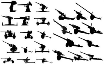
a) Fixed and trailed AWS

b) Self-propelled AWS

Usually, as shown in Fig. 1(b), the cannons in self-propelled AWS [3, 4] are loaded on tracked vehicles while military trucks (MTs) are used to trail such cannons in the battlefield. Now, the MTs are used to load cannons due to the great developments in their capacities and capabilities, in addition to the new generations of strong traction motors. The advantages of using MTs to transport cannons can be summed up in; the high-speed mobility, rapid deployment, and AWS cost reduction. The MTs which used to transport cannons have many added parts such as tilting legs, gun housing, gun frame, ammunition housing, bombardment, etc. By virtue of the MT works in the battlefield, it must be more rigid and more reliable comparing with the civilian one. Also, the weight must be decreased to the minimum level to guarantee the mobility and maneuverability. The most difficult challenge in the design of these MTs isn’t just the vehicle capacity or the ability to carry and transfer the cannon system, but it is how to resist the strong launch forces without dominant vibration during the launching phase or rapid deterioration in the AWS total efficiency. Thus, in the case of truck-mounted howitzer, usually the designers use the instillation legs as a weapon system aids during launching phase to increase the system resistance against the launch vibration dynamics. Since the Second World War until now, there are different countries that have worked and created different types of these AWS [2]. They have researched to load the different types of cannons on the MTs as presented in Table 1.

The muzzle disturbance has a great influence on the firing accuracy. More prosaically, just an error in the firing angle with about 0.05 degree leads to firing dispersion in range 5 km with about 25 meters. In case of gun loaded on MTs, the muzzle disturbance is generated mainly due to two main factors. The first is basically due to the flexibility nature of the long length barrel; while the other is due to flexibility nature of the whole AWS structure especially the truck main chassis [6-9]. This chassis design must be improved to resist the huge launching force and to guarantee the high-speed mobility with more reliability. The rigidity of the chassis can be increased by improving the material properties or by increasing the thickness of chassis main parts under the weight constraints. Thus in practice, the trend of increasing chassis stiffness by adding structure to the MT is avoidable choice.

There are a lot of studies that deal with launch vibration reduction to decrease the Muzzle Disturbances (MD) [10-13]. Most of them can be summarized in two basic trends; firstly, improving the MD through evolving the performance of the recoiling system, and the other trend is to improve the MD by adding some structure to AWS to increase its rigidity or by applying optimization techniques to ameliorate the system layout. Actually, most of these studies simulate the MD from the point of view of cannon structure flexibility modeling but there are few studies that deal with the MD simulations from the point of view of carrier structure flexibility modeling.

In this article, sensitivity analysis of Multi-body Dynamic Model (MBDM) which simulates launching is applied to identify the critical design parameters that affect the MD and to specify the simulation ranges for them. In addition, it assists the designer to examine the possibility of incorporating a hydraulic control circuit to the weapon system in order to control the launching vibration. It is planned that this hydraulic control circuit will consist of two hydraulic cylinders instead of side instillation legs.

2. Recent studies of using multi-body dynamic techniques in AWS design

In fact, it’s important to provide a simplified definition for the gun launch dynamics to clarify the main idea and the problem outlines. Simply, the gun launch dynamics can be defined as gun relative motion due to the breech force and its reaction forces beside other forces resulted from the specific tasks as muzzle break force, control force, etc. So, the gun exposes mainly two different types of forces; breech and reaction forces. Most of the reaction forces will be concentrated in the gun recoiling system and in the AW deployment system (instillation feet). Actually, there are a lot of components, within the cannon system, transmit these forces. Hence, a lot of calculations for load transmission and Degree of Freedom (DOF) definitions are needed to complete kinetic presentation of MBDM.

Yu Hailong and Xiaoting Rui [12] generated a new theory by studying multi-body system dynamics which represents certain AWS. They developed field transfer matrix of an arbitrary rigid body vibrating in the linear range and the transfer matrix method of multi-body system. Also, they studied the natural vibration of a general multi-body gun system. They also construct the transfer equation and transfer matrix of the corresponding multi-body gun system, then the analytical form of frequency equation and modal function of the system are developed.

Based on simplifying the structure of towed howitzer, ShiYongsheng, and others [13] built three dimension finite elements analysis model of whole towed howitzer by using finite elements method. They apply completely analyses structure stress and strain of towed howitzer to find out the AWS dangerous points on the condition of static shooting with maximum payload. They also calculate the frequencies and mode shapes of gun tube and system trial.

The dynamic model of the complicated naval gun system was established by SHI Yue-dong and WANG De-shi with Gauss minimum constraint method based on the rigid multi-body dynamics theory [14]. They calculated numerically the fire process of the whole gun system by combining it with correlative experiment parameters. The result indicates that the desk stiffness is a main factor affecting the gun vibration. Therefore, they designed a suitable elevating mechanism that can effectively improve the vibration performance of the tube.

A planar vertical truck model with nonlinear suspension and its multi-body system formulation are presented by B. Simeon, F. Grupp, C. Fiihrer, and P. Rentrop [15]. They created complete system of equations of motion for the truck model consists of a system of differential algebraic equation [16, 17]. All equations are given explicitly, including a complete set of parameter values, consistent initial values, and a sample road excitation. Thus, the resultant truck model allows various investigations of the specific differential algebraic equations effect. Also, this model represented a test problem for the algorithms in control theory, mechanics of multi-body systems, and numerical analysis.

Ahmed Nadeem, and others [18] built a 3-D finite element model of a large caliber gun system using “ANSYS” as s commercial software. Also, the gun dynamics during the firing cycle was simulated to study and predict the effects of various design factors on the dynamic response. They modeled the physical contact conditions of the gun system components using contact technology in ANSYS. Also, they compared the results with general responses of the gun system obtained through available document sources.

3. System composition of the artillery weapon case of study

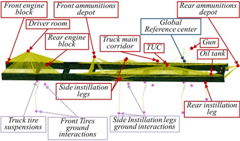
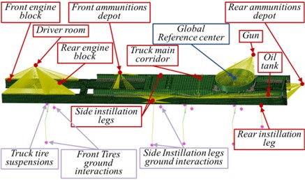
This AWS case of study is used to load 122 mm howitzer cannon on a compatible 6×6 heavy-duty MT as shown in the virtual model presented in Fig. 2(a). A geometrical 3D model of the MT is created by “Creo/Parametric 2.0”, presented in Fig. 2(b). This AWS mainly consists of; 122 mm howitzer cannon, aiming mechanisms, front and rear ammunition reloads and charge system, hydraulic deployment system including 3 fixation legs, gun equilibrator, beside heavy-duty 6×6 special purpose MT including driver and control room, traction motor with front and back engine blocks, truck lower and upper chassis, truck main corridor, tires and main axes, suspension system, fuel and oil tanks. However, due to weight constraints, load distributions, and cost considerations, the MT chassis structures are not made more rigid than necessary, so the truck chassis are assumed to be most dominant flexible component compared with other carrier components. In order to unify the system definitions for all constructed simulations, the selected coordinate system that used to represent both kinetics and kinematics is presented in Fig. 2(b).

Fig. 2AWS case of study

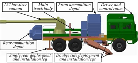
a) 3D model of the whole AWS

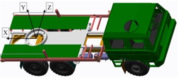
b) 3D model of the carrier MT

4. Complete dynamic model creation for the AWS case of study

To create an accurate MBDM reflects the reality and guarantee the result accuracy, there are different important stages need an intensive care in both definitions and implementations. These stages, with neglecting of the arrangement, are; external applied load definitions; connection definition between different components especially the contact area between such components, DOF definition for each component, and such constraint which must be defined clearly referring to the selected frame of reference. After correcting definitions for all of these stages, the other stages will be easy and simple to be created. The complete building stages for the required MBDM will be defined in detail as follow.

4.2. Firing loads (excitation) measurements and definitions

As a result of simulation complexity of the combustion and ejection process, all firing forces calculations need experimental works in order to validate the results. Due to choosing MT as a point of interest, the center of the upper chassis ring which is used to surround the gun spindle is selected as the point of applied forces and the global reference position as shown in Fig. 2(b). Therefore, all measurements are calculated referred to this point. Under the pre-defined coordinate system, the excitation loads determined from these measurements are portrayed in Fig. 3 as a dotted line. Actually, to measure the pure values for such loads and to avoid the frequency interferences resultant from system flexibility nature, these loads were measured on certain strong test cannon by means of strain gauges during 0.1 sec. The experiment constraints definition will be explained latterly. The sampling rate has been 50 [kHz] which provides 0.02 [ms] as the time between samples. The forces and moments are not completely vanished after 0.1 sec but they decrease sharply after released all combustion gasses at the end of 0.1 sec. Thus, the reminder part of launching load will be ignored. Noting that, these forces and moments are calculated in the case of firing angle zero, because the firing reaction longitudinal loads are in the maximum level at this angle.

The measuring data are difficult to import in the MBDM due to the fixed step time which produces a constraint on the solutions. To avoid this problem, curve fitting algorithm [30-32] was applied searching for the optimal model with maximum simplifications to simulate all launching reaction loads through “Adams” programs. The solid lines presented in Fig. 3 are used to represent such curve fitting. These curves fitting explanation will be omitted to avoid article focusing lost. After examining Fig. 3, it’s important to note that the maximum dominate force is in $X$ direction, dominate moment is around $Z$ axis, and moment around $Y$ axis can be neglect. Noting that, the maximum dominate force direction can be changed by changing the firing angle, while moment around $z$ axis remains in same direction.

Fig. 3Measurements and curve-fitting of launching reaction loads related to the global reference frame

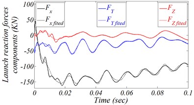
a) Forces

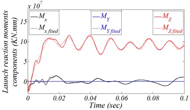
b) Moments

4.3. Dynamic flexible parts generation

Different techniques can be used to create flexible components in MBDM starting from continuous flexible part to discretized finite element part [25-28]. In the majority of MBDM literature on floating, corotational, and inertial frame approaches, the flexible components are discretized using the Finite Element (FE) method. Other discretization techniques have been used in conjunction with the floating frame approach. To simplify the FE model created for the flexible components, all defined materials will be isotropic and homogenous obey hooks law.

As previously mentioned, the flexibility of the cannon carrier can increase the MD, especially the main longitudinal components like the truck main chassis. This truck chassis case of study is divided into 2 main parts; Truck Lower Chassis (TLC), and Truck Upper Chassis (TUC). The detailed geometries and structures for chassis components will be explained latterly. As following, different flexible FE models are created and examined for the truck chassis as a preliminary step in order to be integrated with the MBDM to demonstrate the impact of different flexibilities behaviors of the truck chassis on the numerical simulation results. The construction procedure of a flexible model for different truck chassis components will be explained separately and minutely.

4.3.1. TLC flexible model creation

The main geometric features of the TLC are presented in Fig. 4. TLC consists of longitudinal and crossing U shape axis of symmetric steel beams with the main dimension about 11 mm. Usually, the geometrics of TLC is similar to the traditional civilian heavy-duty truck chassis [29, 30] but it must be more rigid to guarantee the military requirements. In order to guarantee the results accuracy and reliability of the constructed FE model, professional meshing software “Hypermesh” is applied to build the flexible TLC structure.

Fig. 4TLC 3D geometric model

Different types of elements can be used to create the flexible model of this component. Searching for the best flexible model, both 2-D shell element and 3-D solid element are selected to create two different models with different element numbers to check the effect of element type and number on the simulation numerical results, Table 3 lists such FEM parameters. Also, while building the flexible model of TLC and the complete MBDM of the whole AWS system, the following principles and assumptions must be taken into consideration [31]:

1) The assembly gaps between TLC parts are neglected.

2) The origin of the global coordinate system is in the center of the upper chassis ring as shown in Fig. 2 (b).

3) The definition of the modulus of elasticity of the truck components materials, Poisson’s ratio, and material density uses the following units: Length [mm], mass [Ton], density [Ton/mm³], force [N], stress [MPa], angle [Degree], and time [s].

4) The material that has been defined for TLC model is homogenous and linear elastic isotropic obeys Hooks Laws with properties ($\rho =$ 7.85e-9, $E=$ 2.1e5, $\upsilon =$ 0.29).

5) The extended surfaces welding will be simulated by a similar thickness material slice with the same material properties.

6) The assembly of different AWS components on the truck chassis will be constructed by rigid connections between the components CG and the flexible part nodes based on the contact area in the real world.

Table 3Different cases for the constraints definition

	Assembly	Components	Elements	Rigid element	Nodes	DOF	Material
Shell element model	3	21	59,224	39	57,228	343,188	1
Soild element model	3	19	21,651	30	39,721	237,606	1

To create the complete FE model acceptable for modal analysis calculation [32, 33], all AWS components are added to the FEM as a concentrated point masses with inertia tensors which calculated w.r.t the unified frame of reference. Noting that, most of AWS assemblies’ mass properties are measured from the real world or calculated by “Creo/Parametric 2.0”, in which some of MT components mass properties are presented in Table 4. In fact, some assemblies’ properties are omitted in Table 4 like tires, tire axes, and suspension system because the masses of these assemblies are quite small comparing with the other assemblies. Despite of this, all of these mass properties are added to the MBDM to increase the result accuracy. Also, the measured inertia tensors for all assemblies are not presented in Table 4 to avoid the non-beneficial stretching, but their values are constructed accurately in the MBDM.

Table 4Mass properties for some AWS assemblies; Mass [tonn], Distance [mm], I [tonn∙mm2]

Assembly name	C.G position			Mass
	$X$	$Y$	$Z$
Lower chassis (TLC)	–2047	–411	0	0.61
Upper chassis (TUC)	–563	–162	0	0.533
Cannon system	500	666	18	2.482
Driver room	–5027	306	6	1.3081
Truck main corridor	–881.8	–16.32	–7.43	0.329
Front ammunition depot	1720	–149	4	3.048
Rear ammunition depot	–2891	142	35	1.44
Front engine block	–5717	–133	0	0.317
Rear engine block	–4443	–179	0	0.935
Oil tank	979	–396	194	0.12
Fuel tank	–3805	–613	–634	0.14

The photo copies of these two flexible FE models seem to be similar to each other, but they are different in element number, and type; Fig. 5 shows the first shell FEM. Also, in order to reflect the reality, all AWS assemblies with CG position are presented in the same figure, in which they are constructed to the TLC by rigid connection. Also, Fig. 5 represents the interaction between the ground and each road wheel, which are modeled as springs and parallel dampers. This interaction can represent the relative linear motion between ground and tires in all directions. Actually, the suspension mechanisms for all tires are simulated in the same way. Finally, the mass of the whole AWS after constructing all AWS components is about 16.5 tons.

Two different flexible MBDM are constructed in “Abaqus” by using different constructed FEM for the TLC structure. Fig. 5 represents the photo copy of the constructed program created by “Abaqus” which consists of; the flexible FE components (green part), assemblies point masses with concentrated mass properties (red circles), reference or firing point (blue circles), suspension simulation, tire-ground interaction simulation, and feet-ground interaction simulation. Noting, all of these suspensions or springs are appearing in solid violet spheres. In order to check the FEM accuracies, a comparison between the simulation modal analysis of the constructed FEM through “Abaqus” and the experimental snapshots will be accomplished.

Fig. 5Dynamic model of the whole AWS with flexible TLC prepared for modal analysis

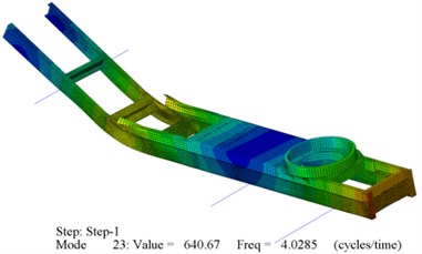
Before studying the modal analysis of the constructed FEM, it’s important to mention that the most important NF that effect the firing accuracy is longitudinal bending. Therefore, the modal analysis research is going to be on this point of interest. The modal analysis numerical results of these two FEM are presented in Fig. 6. These figures represent that the first dominant Natural Frequency (NF) is longitudinal bending with frequency about 4.5 [Hz] which has a great effect on the MD. To verify these results, it is necessary to implement the practical tests to calculate the dominant NF of such AWS [31-33]. These measurements have been implemented carefully to reach the real values of NF, especially in the presence of components more flexible than the rest of the system, like truck tires, which lead to the results overlap. Also there is some avoidable NF related to the rigid manner vibration of the AWS that may cause also results overlap. These experimental specialized modal tests are calculated by certain institute, which confirms that the dominant NF for this AWS is the longitudinal bending with value ${\lambda }_n=$ 4.6 [Hz] which means that the FEM modal analysis results for both models have an acceptable error. Thus both FEM created for TLC can be imported to “Adams” in order to calculate the AWS dynamic response through firing. Of course, the second FEM model for TLC will be the imported model to “Adams” in order to decrease the calculation process time.

Fig. 6Modal analysis results for the whole AWS with flexible TLC

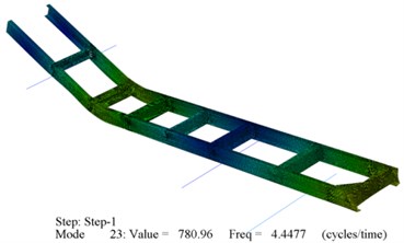
a) Shell element model

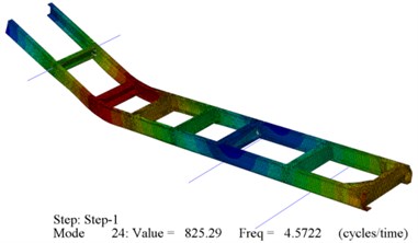
b) Solid element model

4.3.2. TLC, and TUC flexible model creation

The 3D model for both lower and upper truck chassis was depicted in Fig. 7, in which the yellow part represents the TLC, while the gray part represents the TUC. By studying Fig. 8, the difference between TLC and TUC in both shape and configuration is clearly appeared. In fact, TUC consists of; mainly 4 longitudinal U-beams with thickness about 6 mm, 5 crosswise U-beams, 6 inclined assistance U-beams with angle 60, flat cover steel sheet with thickness 4 mm, and a circular ring surrounds the cannon spindle. The generation way to produce the flexible FEM for both TLC and TUC is similar to the way of the TLC with the same principles and assumptions. Different element types will be used to generate the flexible FEM based on the components geometrical shapes.

Fig. 7TLC and TUC 3D geometric model

As shown in Fig. 8(a), the FEM for both TLC and TUC is presented. It’s clear that the FEM become more complicated. The constructed FEM consists of: 27968 solid elements, 9470 shell elements, 279 rigid elements, 64489 nods, 224628 DOF, 5 assemblies, 26 components, 10 properties, and 1 material. Again model analysis will be accomplished to check the accuracy of the FEM numerical results through comparing it with the same experimental results.

Fig. 8a) Dynamic model of the whole AWS with both flexible TLC and TUC; b) Modal analysis numerical results for the whole AWS with both flexible TLC, and TUC

a)

b)

The modal analysis for the whole constructed AWS with both flexible TLC and TUC was presented in Fig. 8(b). The modal analysis numerical results represent also that the first dominate NF is the longitudinal bending with value ${\lambda }_n\approx$ 4 [Hz]. This means that this FEM numerical result has around 8 % error comparing with the experimental results. This error percentage rising, when adding TUC as flexible component, is due to the fact that the average thickness of the TUC is about half the average thickness of the TLC which makes the FEM more flexible. Despite of this result, the resultant error is still in acceptable range. Now, these flexible models are ready for importing in “Adams” to calculate the forced dynamics of the flexible MBDM. Three dynamic simulation programs can be created for each flexible case; rigid, partially flexible, and completely flexible truck chassis. These model numerical results will be used to examine the effect of flexible truck chassis on the MD during cannon firing.

4.4. Multi-body dynamic models constructions

After accomplish all preliminary steps and test the constructed flexible model accuracies, a flexible MBDM will be created through “Adams” software. Fig. 9 shows a complete MBDM planer presentation of the AWS case of study including the global reference, rigidly connected assemblies of the AWS with concentrated masse properties, each of TLC and TUC is presented as thick and dash-dot lines, firing loads with original directions, force elements (dashpots elements), and all the sequence numbers for each AWS assemblies.

Fig. 9Schematic planer presentation for the AWS case of study components assemblies

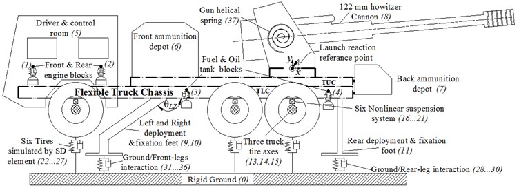
The global base of this DM is the ground which supports and lifts the AWS and it is regarded as an infinity rigid body; numbered as 0. The front engine block, rear engine block, filled fuel tank block, and filled oil tank block respectively are neglected in the drawing because of their complexity shape; numbered as 1-4. In fact, they are added to the MBDM as point masses with their inertia properties. Also, the MT main corridor and outer truck frames are omitted in Fig. 12 to avoid drawing deterioration but its mass properties are added to the MBDM. Actually, all AWS assemblies are added to the DM with a considerable 3-D shape represents the main mass properties in the reality beside both connection type and area with the flexible truck chassis. As an example of these simplifications, driver and control room, ammunition depots, and 122 mm howitzer cannon were added to the MBDM with simplified shapes with guaranteed mass properties; numbered as 5-8. Truck tire axes are simulated as a three constant cylinders diameters with the same mass properties as reality; numbered as 13-15. The suspension system is simulated in the MBDM as a single nonlinear spring for each leaf spring in the reality and it’s an accompanying parallel damper as well ($K_S$); numbered as 16-21. The interaction between tire and ground modeled as a single vertical spring ($K_T$) for each tire, and the accompanying dampers ($C_T$) connect in parallel position; numbered as 22-27. The interaction simulation between the instillation feet and the ground are quite substantial comparing with tire/ground interaction, so these feet are simulated as three Cartesian springs ($K_{fe}$) and parallel accompanying dampers ($C_{fe}$), which can represent relative linear motion in all Cartesian coordinates; numbered as 28-36. The spiral spring ($K_G$) with accompanying spiral damper ($C_G$) are used to connect the canon with the truck chassis to simulate the gun equilibrator; numbered as 37. The MBDM has been constructed with the numerical data presented in Table 5 in addition to all AWS assemblies mass properties presented in Table 4.

Table 5Numerical values used during MBDM creation

Spring element	Value	Dissipation element	Value
$K_S$	90 [N/mm]	$C_S$	0.9 [N∙sec/mm]
$K_T$	10 [N/mm]	$C_T$	1 [N∙sec/mm]
$K_{fe}$	5500 [N/mm]	$C_{fe}$	5.5 [N∙sec/mm]
$K_G$	2×105 [N∙m/rad]	$C_G$	200 [Kg∙m2/s.rad]

In order to check the effect of flexible chassis on the MD, three different MBDM are created in rigid, partially, and fully flexible chassis. These MBDM are presented in Fig. 11 in which; green and red color represent rigid and flexible parts of the chassis respectively, blue color represents gun and ammunition depots. All of these MBDM contain 12 rigid kinematic joints which are used to connect different AWS assemblies, 12 dashpot elements represent the suspension system and tires, 3 reaction force element to represent the reaction forces on the three instillation feet, 3 translational kinematic joints that are used to simulate the truck axes motion during firing, and more than 150 markers operate as a kinematic interface to the different bodies in the MBDM. Finally, 12 dashpot force elements are presented in red color with a spring forms. It’s important to mention that, all the numerical values presented in Table 3 and even the omitted data are completely matched with the numerical data used in modal analysis program for the FEM created before.

Fig. 10Three MBDM for the AWS case of study

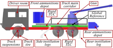
a) Completely rigid chassis

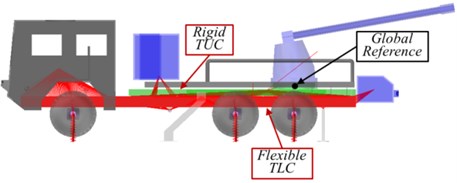
b) Flexible TLC “Partially flexible”

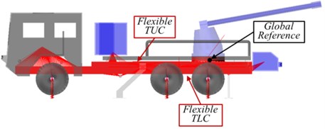
c) Both Flexible TLC & TUC “Completely flexible”

5. Simulation results

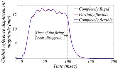
Fig. 11 represent the launch dynamic simulation results for the AWS case study; the black, red, and blue lines respectively represent the three sequential constructed MBDM. By studying these figures, there are some results need to be focused and explained as follow:

1) The total response times for all MBDMs are about 150 milliseconds.

2) The simulation curves are matched in the case of time history for the truck firing reference point displacement magnitude. This is due to that the flexibility nature of the truck chassis does not lead to a significant change in the reference displacement directions.

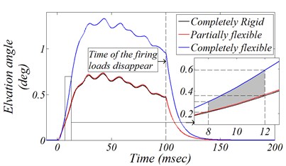
3) The maximum reference displacement is about 13 mm in all MBDM cases, while the maximum elevation angle variation is about 0.6 degree in both cases of completely rigid chassis, and the presence of flexible TLC only. The maximum elevation angle variation is about 1° in case the of completely flexible truck chassis; “approximately twice value”.

4) Fig. 11(b) clearly shows that, the constructing of TLC with the MBDM does not have any considerable change comparing with the response of the totally rigid AWS. This is a logical outcome, due to the large mean thickness of the TLC, about 12 [mm], that is a quite thickness, and due to the rise of rigid interconnection instead of TUC which increases the main rigidity of the chassis.

5) In the case of adding TUC to simulate the complete flexible chassis, the gun elevation angle variation increases approximately twice because of the mean thickness of the TUC is about 6 [mm], which is about half thickness of the TLC.

6) Actually, the average of the Bullet Passage Age (BPA) in the gun barrel is between 8 to 12 [m∙sec], therefore, the firing angle didn’t be affected by the MD in the whole response time. This BPA period time depends on many parameters; canon caliber, bullet propellant charge, etc. Also, Fig. 11(b) depicts a zoom in time history on this BPA period for the truck elevation angle variation, which approximately covers all different time period cases for 122 howitzer cannons.

7) The MD difference range in the right border, 12 [m∙sec], between the completely rigid truck chassis and the completely flexible truck chassis is about 0.23 degree, while in left border, 8 [m∙sec], is about 0.1 degree. More rigorously, this means that adding the flexibility nature of the AWS carrier increases the MD with about 35 %. This is considered as new information about the MD prediction in the AWS design field. In addition, it helps in the future to predict the required controlled displacement needed in the hydraulic instillation feet to decrease these MD.

Fig. 11a) Dynamic model of the whole AWS with both flexible TLC and TUC; b) modal analysis numerical results for the whole AWS with both flexible TLC, and TUC

a)

b)

6. Dynamic model design variable sensitivity

Sensitivity analysis (SA) has spread applications in the engineering optimization scope, especially in the AWS designs. It compels the decision maker to identify the critical variables that affect the stability of AWS, especially at launching phase. Also, the SA indicates the critical variables for which additional information can be obtained for future upgrade design [34]. The main problem in SA is that it doesn’t provide clear cut results it just leads the designer to the suitable design. Three different design variable sets will be selected and examined separately as an input variation of AWS design to investigate their impacts on the MD variations. These sets were classified based on the stability design experience for such AWS family. The following section will represent the effect of these variables on the MD especially in the BPA period, and particularly on left and right borders of the BPA period.

6.1. Set of system stiffness impacts

The first set of design variables is the studying of different soil or ground type effects on the MD, which is in contact with the instillation legs and tires. Simply, different ground conditions mean different connection stiffness between both instillation legs and truck road wheels with the ground. Thus, as the first set, Leg/Ground interaction in both stiffness and damper are tested separately to get a clear investigation of such interaction variation effects on the MD. Extended range of this interaction stiffness values $K_{fe}=$ 1-10 [KN/mm], were examined at constant Leg/Ground damping value, $C_{fe}=$ 50 [N∙sec/mm]. The resultant effects of these design variables on the maximum absolute value of the MD and in both left and right borders of BPA are presented in Fig. 12, respectively.

Noting that, based on the nature of this AWS family, the stability during launching is established mainly by the instillation legs, thus, the effect of Tire/Ground interactions variation in both stiffness and damping value is too weak and the resultant SA for this design variable will be ignored. Under the same basis, the same results can be concluded with the study of truck suspension stiffness and damping values variations.

By studying Fig. 12(b), it’s clear that the elevation angle disturbance in both BPA border increase rapidly after $K_{fe}$ simulation value less than 5 [KN/mm]. Actually, in the case of $K_{fe}$ more than 5 [KN/mm] the MD decreases sharply and the variation effect of this design variable seems to be vanished. Thus, as a first conclusion, the Leg/Ground stiffness simulation values must be greater than 5 [KN/mm] which reflects on the reality of the zodiac design of the instillation leg. Thus, this mere fact must be taken into consideration during the implementation of the upgrade expectation design for such weapon system. Commonly, the variation of the damping value didn’t have a significant effect on the maximum value of the MD as shown in Fig. 12(b), but actually, it can affect the transient response behavior which will affect the MD on the BPA borders as shown in Fig. 12(a). This figure shows that, the simulation damping value must be around 5 [N∙sec/mm] to prevent undesirable MD peaks on the BPA borders.

Fig. 12Effect of Leg/Ground interaction stiffness and damping variation on the muzzle disturbance

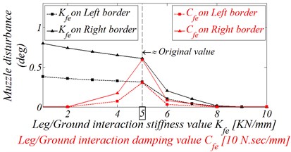
a) Muzzle disturbance on the BPA borders

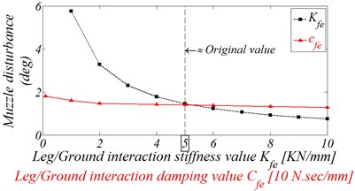
b) Absolute maximum muzzle disturbance

6.2. Set of instillation legs configuration parameters impacts

The installation feet in this AWS type are considered as the most responsible components for the system stability during firing. Therefore, different parameters for the instillation feet will be studied and examined separately to investigate clearly the effect of these parameters on the MD. In fact, this study will complement all requirements of SA for this component, because it will be a part of the future upgrading. As a general rule, the original values of these feet always lay in the middle of any variation and the resultant SA will be explained through representing the MD maximum value and the MD on the BPA borders.

Often, the side legs are designed at angle against the direction of the launching reaction forces to increase their resistance capabilities against the firing load and to reduce the firing stresses. Mainly, this angle consists of two parts; the first part is a rotating angle of foot main axis about $Z$ axis (${\varphi }_{feZ}$), while the second part is a rotating angle of foot main axis about $Y$ axis for both left and right legs (${\varphi }_{feY}$), more precisely, it is the angle between the vertical truck side and the foot main axis. Logically, any increase in both types of leg angles leads the system to become more stable and MD must be decreased.

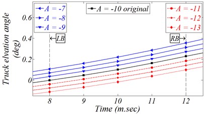
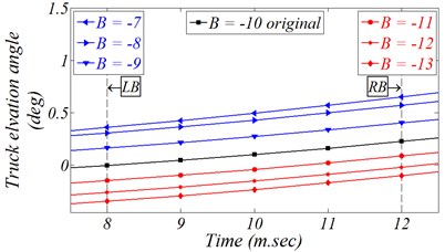
The variation impacts on the MD of side instillation legs; lateral positions, longitudinal positions, and tilting angles about the global axis $Y$ and $Z$ are examined. Also, the rear instillation leg longitudinal positing, and the general height of the truck from the ground base, which can be changed as a result of the length extracting along instillation feet, are examined. All resultant SA impacts on the MD which applied on the MBDM with completely flexible MT chassis are presented in Table 6. To avoid the difficult reading of this table details and to determine the impact of the individual design parameters for the instillation legs on the MD, Fig. 13 have been implemented to indicate separately the table content. To demonstrate the MD resultant deviation from its original values, as a result of specified variation, both Fig. 15 will represent the original MD values on the BPA borders and the absolute maximum values presented as a horizontal thin dashed line in both figures. To collect all results in the same figure, the values of the $X$ axis on this figure are the parameter variations for each design variable individually with the same order as presented in Table 6.

Table 6Sensitivity analysis for the design configuration parameters of the instillation fe

Design parameter	Value	Maximum MD	Left border MD	Right border MD
Side legs deployment lateral position variation ($f{e}_Z$) [mm]	100	1.334	0.308	0.589
	Original-200	1.334	0.316	0.595
	300	1.334	0.306	0.589
	400	1.335	0.317	0.596
	500	1.335	0.305	0.589
Side legs deployment longitudinal position variation ($f{e}_X$) [mm]	–450	1.196	0.297	0.552
	–300	1.234	0.3	0.564
	–150	1.301	0.302	0.581
	Original-0	1.333	0.306	0.592
	+150	1.426	0.311	0.622
	+300	1.486	0.321	0.641
	+450	2.349	0.328	0.657
Side legs deployment angle variation around $Z$ axis (${\varphi }_{feZ}$) [deg]	0	1.78	0.341	0.723
	10	1.68	0.333	0.693
	20	1.59	0.326	0.666
	30	1.49	0.318	0.639
	Original-40	1.33	0.311	0.611
	50	1.30	0.304	0.582
	60	1.19	0.297	0.55
Side legs deployment angle variation around $Y$ axis (${\varphi }_{feY}$) [deg]	Original-0	1.333	0.306	0.592
	5	1.325	0.302	0.588
	10	1.319	0.291	0.583
	15	1.31	0.282	0.582
	20	1.25	0.26	0.581
Back leg longitudinal position variation ($B_{feX}$) [mm]	–450	1.196	0.297	0.552
	–300	1.234	0.3	0.564
	–150	1.292	0.303	0.582
	Original-0	1.333	0.306	0.592
	+150	1.50	0.302	0.565
	+300	1.486	0.321	0.621
	+450	1.55	0.328	0.607
General truck mounted howtizer height ($TM{H}_Y$) [mm]	1200	1.277	0.302	0.574
	Original-1300	1.333	0.306	0.592
	1400	1.433	0.315	0.624
	1500	1.525	0.324	0.654
	1600	1.625	0.335	0.686

By studying the majority presentation of Fig. 13, the following conclusions can be formulated:

1) Side legs deployment lateral position variation ($f{e}_Z$), and angle variation around $Y$ axis (${\varphi }_{feY}$) have a weak effect on the MD of the BPA borders and even on the maximum absolute value of the MD. These results are logic because of by revising Section 4.2, it’s clear that the lateral reaction force ($F_Z$) is too small comparing with the other reaction forces components, also the same phenomena can be found in the reaction moments where ($M_Y$) is almost at zero level.

2) The parameter of back leg longitudinal position ($B_{feX}$) has a moderate resultant effect on the maximum absolute value of the MD, which in fact didn’t affect the firing accuracy as a result of BPA, but it has little effects on the MD on BPA borders especially at the extreme values of the parameter variation.

3) As the first parameter that has a significant effect on the MD deviation on the BPA borders, the general weapon system height ($TM{H}_Y$) increases MD by10 % on the right border. Actually for different purposes, the general height from the ground is always chosen to be at the minimum level.

4) The studying of longitudinal position variation for side deployment legs with respect to original position ($f{e}_X$) shows, if the longitudinal position of the side legs has changed by about 400 [mm] in the negative direction of the global axis $X$ the MD in both BPA borders will decrease about 11%.

5) The most dominate DV effect the MD is the side legs deployment angle variation around $Z$ axis (${\varphi }_{feZ}$). The approximately linear relation between this angle and the MD are shown clearly. Simply, just an increase in this angle by 10° will decrease the MD in the BPA border by 5 % and on the absolute maximum value of the MD by about 10 %.

Fig. 13Effect of all design parameters of the instillation legs on the MD

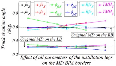
a) Resultant MD on the BPA borders

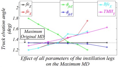
b) Absolute maximum MD

7. Set of artillery weapon system structure layout impacts

As mentioned before this AWS consists of many components assemblies. The strangest components that disappeared in the other AWS types are the front and back ammunition depots. Therefore, both longitudinal and height position variations for these depots are examined to study their effect on the MD. The results prove that these design variables don’t have a dominant effect on the MD; about 0.5 % at the most and at the extreme position. This is because of the limited available position variation space for these parts and due to the weight of these parts is not big enough compared with other parts of the system.

8. AWS Future upgrade modification

By studying this AWS launching dynamics beside the applied SA, it’s clear that the MD cannot be reduced significantly or completely controlled through the traditional methods of optimizations. Therefore, a feature opportunity idea of adding a hydraulic system to decrease the MD arises. Hence, the question appears; “what will happen in the MD if, the length of the side installation legs changes especially in $Y$ direction through the firing phase?”. In fact, these legs will be exchanged by hydraulic cylinders that can withstand strongly the firing loads and perform a schedule kinetic scheme during firing via electrohydraulic servo controller. The answer needs to examine two major ideas; the first is whether the system performance will improve or would lead to a partial collapse, and the other is in case of performance improving, the assistance hydraulic system can perform this relatively fast-acting response compared with the general applications of hydraulic systems. To formulate these ideas, the main problem will be divided into 2 main parts based on the previous explanation. The first part is to identify clearly the predefined schedule kinetic scheme needs to be applied during the firing phase and this will be the next scope, and the second part is the design on this circuit.

The required kinematic scheme can be expected through reexamining Fig. 11(b), and studying Fig. 14, which show the displacement time histories and the launching reaction forces for this AWS side legs connection points in $Y$ direction. In fact, these points are the connection between the truck side chassis body and the side legs main body. By studying these figures, it’s clear that the displacement and forces for both left and right legs seem to be similar in both total response behavior and main values.

Based on this similarity, one of them is chosen to be the opposite displacement required from the hydraulic cylinder in which the reaction forces will be the applied disturbance. A proposal of Gaussian curve for this displacement, as a position envelope enclosing the resultant displacement of the connection point of the fixation leg, is presented also in Fig. 14(a) based on Eq. (2). Where, $HDP$ is the cylinder position, $t$ is the independent time variable, and ($A$, $\mu$, $B$) are the Gaussian curve parameters whose values are presented in the same figure. Both parameters $A$ and $B$ can control the amplitude and the width of this kinematic proposal:

Fig. 14Side legs connection points

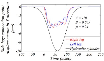
a) Displacement

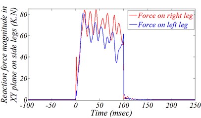
b) Reaction force magnitude in $XY$ plane

Fig. 15Effect of predefined schedule kinetic scheme applied through instillation side legs

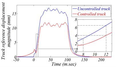
a) Reference displacement magnitude variation

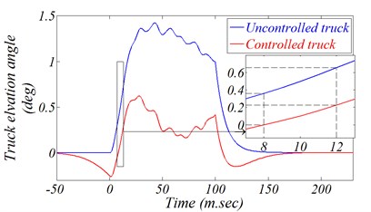
b) Firing angle variation

The effect of incorporating this proposal displacement on both AWS reference displacement magnitude and firing angle variation is presented in Fig. 15). These figures show that this proposal has an obvious effect on system response, which decrease the truck reference displacement magnitude and MD on the BPA borders by about 50 %. More clearly, the MD can be decreased on the left border to 0° which mean that the MD can be controlled completely until reaching a certain value determined by the designer in advance.

Different Gaussian parameters are tested to investigate their impacts on the MD, and to examine the system capabilities to withstand these parameters variations without any deteriorations in the major performance. The linearization effect of these parameters on the MD is clearly approved by studying Fig. 16. Thus, the designer can choose the best kinematic profile required to guarantee the minimum level of the MD.

Fig. 16Effect of different control action on AWS response

a) Reference displacement magnitude variation

b) Firing angle variation

9. Conclusions

For cannons loaded on the MT, the truck chassis is considered as the dominant flexible part affects the MD. This article has focused on studying the impact of the integration of flexible chassis with AWS loaded on a specific truck on the MD. The flexible chassis model has been built to possess the properties of the real world in both geometry and material properties. The chassis flexible model is verified through a practical modal test. Different types of flexible chassis effect on the MD have been examined in either complete or partial flexible components. The influence of the presence of a completely flexible truck chassis on the AWS doubles the MD compared with the completely rigid AWS. The sensitivity analysis has been examined for different DV, to investigate the best design parameters and to decrease the MD. A future generation of this AWS incorporated with an assistance electrohydraulic control circuit is examined in different cases in order to test the ability to decrease the MD to the minimum level in case of fully control AWS. Finally, this paper provides the theoretic basis for the system design, dynamic analysis, and finalizing the layout of the truck mounted howitzer.