Resonance response analysis of the slab track caused by moving vehicle

1. Introduction

The slab track is widely in service for metro and high-speed railway in China, Europe, USA and Japan. Slab track basically consists of concrete slabs supported on resilient elements such as cement asphalt mortar, rubber bearings. Dynamic response between vehicle and slab track turns to be more obvious because slab track has higher stiffness. Violent track vibration will cause track damage and shorten service life.

Therefore, great efforts have been attached to dynamic response of slab track in recent years. Zhu et al. [1] carried out dynamic analysis of vehicle–slab track (CVST) systems by means of a vehicle-track coupling dynamic model considering nonlinear and fractional derivative viscoelastic (FDV) of rail pads. Zhai et al. [2] developed a three dimensional vehicle-track coupled dynamic model in which the non-ballasted slab track is modeled as two parallel continuous beams supported by a series of elastic rectangle plates on a viscoelastic foundation. The vehicle-track coupled model has been validated by full-scale field experiments, showing good correlation between theoretical and experimental results. Kuo et al. [3] analyzed effects of slab bearing on track responses by coupled equilibrium equations of suspended wheels and floating slab track system. The correlation between wheel-rail resonance and train speed was also discussed. Steenbergen et al. [4] carried out a parametric study on the slab track on soft soil from a dynamic viewpoint. The classical model of a beam on elastic half-space subject to a moving load is employed to simulate slab vibration.

However, those studies focus on deflection and vibration analysis of track and vehicle, and running safety of vehicles on various slab tracks is examined. What condition will lead to track resonance remains unresolved. So far the major finding has been so-called ‘critical speed’ at which the speed of the moving force would equal to that of wave propagation in the beam. This critical speed is usually greater than 1000 km/h for general track and is far beyond the speed of present and foreseen [5]. But the critical speed may just have academic interest for railways.

For the present train speeds it may take some sense to take into account the discrete feature of rail supports in investigation of wheel-rail resonance. This is because track structure resonance cause damage to rail and car shaking, although train running velocity is low.

Due to the complexity of track structure vibration, relatively few works have been conducted to consider resonance mechanism and conditions of slab track system. This paper focuses on dynamic response of the slab track systems of railway under the action of vehicles. The vehicle-slab track coupling model and moving sprung mass model on slab in this paper can be used to simulate the vehicle and slab track interaction at any speed. The resonance mechanism and conditions of slab track system are investigated through theoretical derivations and numerical simulations. In a numerical case study, the effect of rail pad stiffness and slab bearing stiffness on resonance phenomena of track system are analyzed. This study may help to clarify some questions mentioned above.

2. Analysis model

2.1. Dynamic analysis model of vehicle-slab track

2.1.1. Motion equation of vehicle model

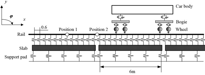
The vehicle subsystem involves a car body and two bogies. The car body, the front and the rear bogies are each assigned two DOFs: vertical and pitch motion. Then the vehicle subsystem is modeled as a multi-body system with 6 degrees-of-freedom (DOFs) running on the track with a constant velocity, as shown in Fig. 1.

The equations of motion for vehicles can be obtained according to the D’Alembert’s principle. It can be written as:

1

$M_v\ddot{u}+C_v\dot{u}+K_{v}u=F_v,$

where $u\text{,}$$\dot{u}$ and $\ddot{u}$ denote the displacement, velocity and acceleration vectors of vehicle. The displacement vector of the vehicle is given by:

2

$u_v=\left[\begin{array}{llllll}{z}_c& {\phi }_c& z_{t1}& {\phi }_{t1}& z_{t2}& {\phi }_{t2}\end{array}\right],$

where $z_c$, $z_{t1}$, $z_{t2}$ denote the vertical displacement of the car body, the front and rear bogies respectively, ${\phi }_c$, ${\phi }_{t1}$, ${\phi }_{t2}$ denote the pitching rotations of the car body, the front and rear bogies respectively.

$M_v$ is mass matrix of vehicle, the mass matrix can be written as:

3

$M_v=\mathrm{D}\mathrm{i}\mathrm{a}\mathrm{g}\left[\begin{array}{llllll}{m}_c& r_c& m_{t1}& r_{t1}& m_{t2}& r_{t2}\end{array}\right],$

where $m_c$, $m_{t1}$, $m_{t2}$ denote the mass of the car body, the front and rear bogies respectively, $r_c$, $r_{t1}$, $r_{t2}$ denote the rotator inertia of the car body, the front and rear bogies respectively.

$K_v$ is stiffness matrix of vehicle, the stiffness matrix can be written as:

4

$K_v=\left[\begin{array}{cccccc}2k_{tz}& 0& -k_{tz}& 0& -k_{tz}& 0\\ 0& 2l_c^2{k}_{tz}& l_c{k}_{tz}& 0& l_c{k}_{tz}& 0\\ -k_{tz}& l_c{k}_{tz}& k_{tz}+2k_{pz}& 0& 0& 0\\ 0& 0& 0& 2l_t^2{k}_{pz}& 0& 0\\ -k_{tz}& l_c{k}_{tz}& 0& 0& k_{tz}+2k_{pz}& 0\\ 0& 0& 0& 0& 0& 2l_t^2{k}_{pz}\end{array}\right],$

where $k_{tz}$ is vertical stiffness of secondary suspension system, $k_{pz}$ is vertical stiffness of suspension system, $l_c$ is half length between truck centers, $l_t$ is half of wheelbase.

The damping matrix $C_v$ can be obtained by simply replacing the variant “$k$” in the matrix $K_v$ by “$c$”.

$F_v$ is the vector of loads acting on the vehicle, the vector can be written as:

5

$F_v={\left[\begin{array}{c}-m_{c}g\\ 0\\ -m_{t1}g+k_{pz}(z_{w1}+z_{w2})\\ -l_t{k}_{pz}(z_{w1}-z_{w2})\\ -m_{t2}g+k_{pz}(z_{w3}+z_{w4})\\ -l_t{k}_{pz}(z_{w3}-z_{w4})\end{array}\right]}^T,$

where $z_{wi}$ is vertical displacement of the $i$th wheel.

Fig. 1Model of vehicle on slab track

2.1.2. Equation of slab track

In this paper, only the dynamic behavior in the vertical plane is studied, but the axial deformations of rail and slab are neglected. Both the rail and slab are modeled as a uniform Bernoulli-Euler beam. The rail is considered as beam with discrete continuous elastic supports resting on slabs, and the slabs are regarded as beams with free ends on continuous supporting foundation, as shown in Fig. 1.

The model of track is obtained using finite element method, and written as:

6

$M_r\ddot{q}+C_r\dot{q}+K_{r}q=F_r,$

where $q$ denote displacement vector of beam element nodal, and can be written as:

7

$q=\sum _{i=1}^{NE}{q}_i^e,$

8

$q_i^e=\left[\begin{array}{llll}{y}_{2i-1}& {\phi }_{2i}& y_{2i+1}& {\phi }_{2i+2}\end{array}\right],$

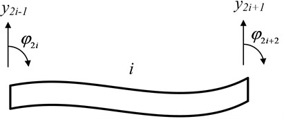
where, $q_i^e$ is displacement vector of the $i$th element nodal, $NE$ denotes number of elements, $y_{2i-1}$, $y_{2i+1}$ are vertical deflection of the (2$i$)thand (2$i+$2)th element nodal, ${\phi }_{2i}$, ${\phi }_{2i+2}$ are rotation of the (2$i$)th and (2$i+$ 2)th element nodal, as show in Fig. 2.

Fig. 2Beam element

$M_v$ is mass matrix of track, and may be expressed as:

9

$M_r=\sum _{i=1}^n{m}_{rail}^e+\sum _{i=1}^n{m}_{slab}^e,$

10

$m_{rail}^e=\frac{m_{r}l}{420}\left[\begin{array}{cccc}156& 22l& 54& -13l\\ 22l& 4l^2& 13l& -2l^2\\ 54& 13l& 156& -22l\\ -13l& -3l^2& -22l& 4l^2\end{array}\right],$

where, $m_{rail}^e$ is mass matrix of rail element, $l$ is element length, $m_r$ is mass per unit length of rail.

$m_{slab}^e$ is mass matrix of slab element. Its expression is much similar to $m_{rail}^e$. We can obtain $m_{rail}^e$ by replacing $m_r$ in $m_{rail}^e$ by $m_s$:

11

$K_r=\sum _{i=1}^n{k}_{rail}^e+\sum _{i=1}^n{k}_{slab}^e.$

$k_{rail}^e$ is stiffness matrix of rail element, and can be written as;

12

$k_{rail}^e=EI\left[\begin{array}{cccc}12/l^3& 6/l^2& -12/l^3& 6/l^2\\ 6/l^2& 4/l& -6/l^2& -2/l\\ -12/l^3& -6/l^2& 12/l^3& -6/l^2\\ 6/l^2& 2/l& -6/l^2& 4/l\end{array}\right],$

where $E$ is rail bending stiffness, $I$ is rail bending moment of inertia.

$k_{slab}^e$ is stiffness matrix of slab element, and can be written as:

13

$k_{slab}^e=\frac{k_{c}l}{420}\left[\begin{array}{cccc}156& 22l& 54& -13l\\ 22l& 4l^2& 13l& -2l^2\\ 54& 13l& 156& -22l\\ -13l& -3l^2& -22l& 4l^2\end{array}\right],$

where $k_c$ is coefficient of continuous elastic foundation.

$F_r$ is the vector of loads acting on rail, the vector can be written as:

14

$F_r=\sum _{i=1}^{\mathrm{n}\mathrm{w}}{Q}_p^e,$

15

$Q_p^e=N^T{P}_{wi},$

where $nw$ is number of wheel, $P_{wi}$ is the force between wheel and rail, $N$ is shape functions of beam, and the shape functions may be expressed as:

16

$N_1=1-3{\left(\frac{x}{l}\right)}^2+2{\left(\frac{x}{l}\right)}^3,$
$N_2=-x+\frac{2x^2}{l}-\frac{x^3}{l^2},$
$N_3=3{\left(\frac{x}{l}\right)}^2-2{\left(\frac{x}{l}\right)}^3,$
$N_4=\frac{x^2}{l}-\frac{x^3}{l^2},$

where $x$ is local coordinate measured from left node of the beam element.

2.1.3. The relationship between wheel and rail

Since each wheel is assumed to be always in contact with the rail beam, the motion of wheel can then be written as [6]:

17

$z_{wi}=N{q}_i^e,$
${\dot{z}}_{wi}=N{\dot{q}}_i^e+v{N}^{\mathrm{\text{'}}}{q}_i^e,$
${\ddot{z}}_{wi}=N{\ddot{q}}_i^e+2v{N}^{\mathrm{\text{'}}}{q}_i^e+a{N}^{\mathrm{\text{'}}}{q}_i^e+v^2{N}^{\mathrm{\text{'}}\mathrm{\text{'}}}{q}_i^e,$
$q_i^e=\left[\begin{array}{llll}{y}_{2i-1}& {\phi }_{2i}& y_{2i+1}& {\phi }_{2i+2}\end{array}\right],$

where the dot above symbol denotes differentiation with respect to time $t$, $v$ denotes the vehicle velocity in the longitudinal direction, a denotes the vehicle acceleration in the longitudinal direction, $q_i^e$ is the nodal displacement vectors of rail beam element, shape function $N$ adopts Hermitian cubic interpolation function.

The force between rail and wheel can be expressed as:

18

$P_{w1}=k_{pz}\left(-z_{t1}+l_t{\phi }_{t1}+z_{w1}\right)+m_w{\ddot{z}}_{w1}+m_{w}g,$
$P_{w2}=k_{pz}\left(-z_{t1}-l_t{\phi }_{t1}+z_{w2}\right)+m_w{\ddot{z}}_{w2}+m_{w}g,$
$P_{w3}=k_{pz}\left(-z_{t2}+l_t{\phi }_{t2}+z_{w3}\right)+m_w{\ddot{z}}_{w3}+m_{w}g,$
$P_{w4}=k_{pz}\left(-z_{t2}-l_t{\phi }_{t2}+z_{w4}\right)+m_w{\ddot{z}}_{w3}+m_{w}g.$

Based on the relationship between wheel and rail, the total stiffness matrix, total mass matrix, and total damping matrix for the vehicle and track coupling system can be formulated. The system equations of vehicle and track can be solved by Newmark-$\beta$ method which is used in this study.

Table 1Parameters for the vehicle and track

Item and notation	Value	Unit
Mass of car body ($m_c$)	2.68×104	kg
Mass of bogie ($m_t$)	1600	kg
Mass of wheelset ($m_w$)	1200	kg
Pitch moment of inertia of car body ($r_c$)	1.35×106	kg.m2
Pitch moment of inertia of bogie ($r_t$)	3600	kg.m2
Half-length between truck centers ($l_c$)	8.5	m
Half of wheelbase ($l_t$)	1.25	m
Vertical secondary stiffness ($k_{tz}$)	4×105	N/m
Vertical secondary damping ($c_{tz}$)	5×104	N·s/m
Vertical primary stiffness ($k_{pz}$)	1.04×106	N/m
Vertical primary damping ($c_{pz}$)	4×104	N·s/m
Rail bending stiffness ($E$)	2.059×1011	N/m2
Rail bending moment of inertia ($I$)	3.217×10-5	m4
Mass of rail ($m_r$)	60.8	kg/m
Rail pad spacing ($l_p$)	0.6	m
Stiffness of rail pad ($k_p$)	5.0×107	N/m
damping of rail pad ($c_p$)	7.5×104	N·s/m
Slab bending stiffness ($E_s$)	3.5×1010	N/m2
Slab bending moment of inertia ($I_s$)	4.05×10-3	m4
Mass of slab ($m_s$)	2.5×10-3	kg
Slab length ($l_s$)	6	m
Stiffness of slab bearing ($k_s$)	6.5×106	N/m
Damping of slab bearing ($c_s$)	7.5×104	N·s/m

Parameters for the vehicle and track are given in Table 1. In order to reduce the boundary effects of the track, the total track length is 100 m. All the analyses were done without any consideration on wheel or rail surface irregularities and track system damping in order to accentuate the resonance response causes by track structure flexibility. The rail deformations embodied in this paper are the rail deformations on position 2 (shown in Fig. 1).

2.2. Model of moving sprung mass on slab track

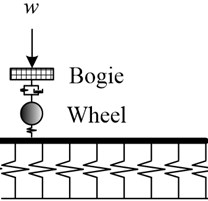
To simplify the vehicle-track model used for the vehicle-track resonance phenomena, a vehicle is model as a sequence of moving sprung masses sustaining a concentrated load lumped from the weight of the car body, as shown in Fig. 3.

The differential equation of motion of sprung mass is:

19

$m_t{\ddot{z}}_t+k_{pz}(z_t-z_w)=-\frac{w}{4},$
$w=m_{c}g+2m_{t}g,$

where $m_c$, $m_t$ denote the mass of the car body, bogies respectively, $z_t$, $z_w$ denote the vertical displacement of the bogies, wheelset respective, $k_{pz}$ is vertical primary stiffness.

Fig. 3Model of moving sprung mass on slab track

3. Loaded track resonant speed

The loaded track frequency $f_{w/t}$ of a coupled wheel-track system on an elastic foundation of uniform stiffness can be approximately estimated by [7-9]:

where $k_{tr}$ and $m_{tr}$ are the effective stiffness and mass respectively, and $k_f$ is the equivalent stiffness per unit length of the elastic foundation.

For a moving wheel-load system with constant speed $v$ travelling along a track supported by discrete rail-pads of constant intervals, the excitation frequency $f_{ext}$ to the wheel-load system due to the discrete rail-pads is:

where $L_e$ is the effective spacing between two adjacent rail-pads.

When the excitation frequency equals the loaded track frequency, resonance can be excited between the bogies and the rails. The resonant speed $v_{res}$ can be solved as:

By substituting the data assumed for the Table 1 into Eqs. (20)-(22), the resonant speeds can be computed, as shown in Table 2.

4. Resonant analysis

Refer to the parameters in Table 1, and the slab bearing stiffness is set as $k_s=$6.5×10⁸ N/m, rail pad stiffness $k_p=$6×10⁷ N/m, the forces between wheel and rail calculated at the speed of 300 km/h, 120 km/h and 50 km/h are shown in Fig. 4.

Fig. 4The time history of forces between wheel and rail at different speed

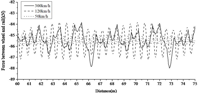
Fig. 5The frequency spectrum of contact force at different speeds

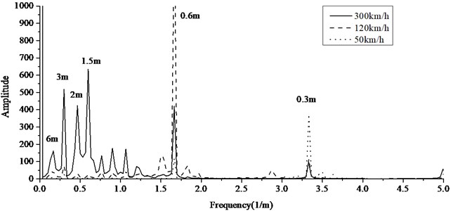
It shows when the speed is low, forces between wheel and rail changes periodically according to the distance of adjacent rail pads. When the speed is high, forces between wheel and rail involve several periodic components according to several factors, such as the distance of adjacent rail pads, slab length, etc. Fig. 5 shows frequency spectrum at different speeds. The frequency component 1.67 Hz (0.6 m) caused by rail pad spacing always exists. Forces between wheel and rail within the frequency of 0-1 Hz account for a large proportion when the speed is high.

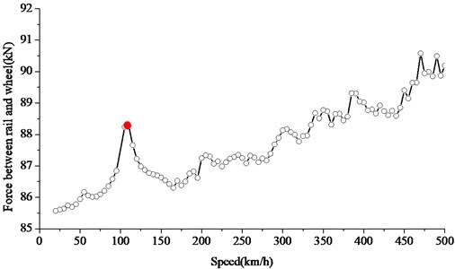
Based on the moving sprung mass model as mentioned in the previous section, the rail deformation and wheel-rail contact force have been plotted with respect to the speed in Figs. 6 and 7. It can be seen that vibration attenuation of slab track is low so the peak resonance is more easily induced and the resonance phenomena will be more obvious. The speeds at which obvious peak rail deformations occur are 108 km/h, 237 km/h, 343 km/h and 480 km/h, and these speeds correspond with the resonance speeds in Table 2 perfectly. The peak forces between wheel and rail at the speed of 108 km/h, corresponding with the first-order resonance speed due to 0.6 m rail pad spacing. As a whole, the first-order resonance caused by rail pad spacing is more obvious. Because the said resonance speed is within the range of normal operating speed, the wheel-rail wear and rail damage may worsen, and it should be emphasized.

Fig. 6Increase of rail displacement based on moving sprung mass model

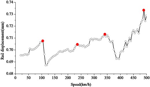
Fig. 7Increase of contact force based on moving sprung mass model

5. Case study

5.1. The effect of stiffness of rail pad

The analysis in this section set the slab bearing stiffness as $k_s=$6.5×10⁸ N/m, rail pad stiffness $k_p=$6.0×10⁷ N/m, $k_p=$7.5×10⁷ N/m and $k_p=$9.0×10⁷ N/m. By substituting the data assumed for the Table 1 into Eq. (20)-(22), The resonance speeds under different rail pad stiffness conditions caused by the 0.6 m interval of rail pad can be computed, as shown in Table 3. It can be seen that with the increasing of rail pad stiffness, the resonance speed increase.

In design practice, the impact factor $I$ is used to account for the amplification effect on the response of the vehicle and track. The impact factor is defined as follows:

23

$I=\frac{R_d\left(x\right)-R_s\left(x\right)}{R_s\left(x\right)},$

where $R_d\left(x\right)$ and $R_s\left(x\right)$ respectively denote the maximum dynamic and static responses of vehicle and track due to the action of the moving loads.

Table 3Resonant speeds of track system under different rail pad stiffness conditions

Rail pad stiffness $k_p$ (N/m)	Resonance velocity (km/h)
	$n=$1	$n=$2	$n=$ 3	$n=$4
6.0×107	116	232	348	463
7.5×107	126	252	378	505
9.0×107	135	270	406	541

Fig. 8Increase of impact factor of rail deflection at different rail pad stiffness

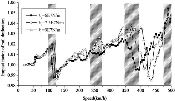
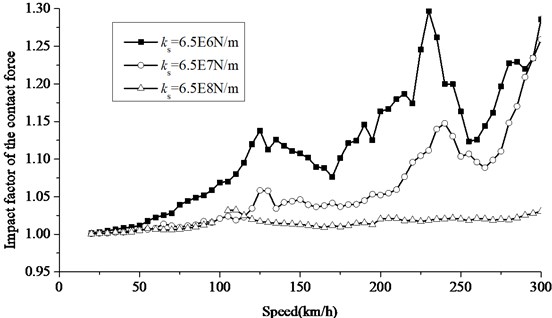
Fig. 9Increase of impact factor of contact force at different rail pad stiffness

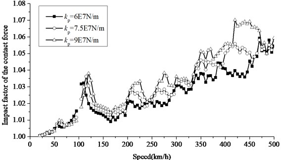
Figs. 8 and 9 shows impact factor of rail deflection and wheel rail contact force in case of different rail pad stiffness adopting the moving sprung mass model. When the rail pad stiffness increase, the wheel-rail resonance tends to be worse to some extent and dynamic response tends to be amplified. The speeds at which peak rail deformation occurs are identical with the resonance speeds due to 0.6 m rail pad spacing in Table 3. Each gray background corresponds to resonant speeds of track system under $n=$1, 2, 3, 4 conditions, respectively. Peak forces between wheel and rail correspond to the first-order resonance speed. The resonance speed of rail deflection and contact force calculated by numerical simulations slightly increase with the increasing of rail pad stiffness.

5.2. The effect of stiffness of slab bearing

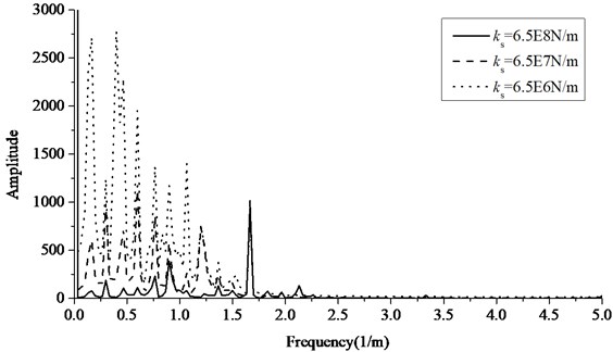
The analysis in this section set the rail pad stiffness as $k_p=$6×10⁷ N/m, the slab bearing stiffness as $k_s=$6.5×10⁸ N/m, $k_s=$6.5×10⁷ N/m and $k_s=$6.5×10⁶ N/m. Fig. 10-11 shows frequency spectrum of force between wheel and rail at the speed of 120 km/h and 200 km/h adopting the moving sprung mass model. At the speed of 120 km/h, the lower the slab bearing stiffness is, the more obvious the 0.17 Hz (6 m) component of wheel-rail force caused by the slab length is. At the speed of 200 km/h, if the slab bearing stiffness is decrease, the 0-1 Hz component of wheel-rail force caused by slab bending is easily inspired and there are several force frequency components. The force frequency component 1.67 Hz (0.6 m) caused by rail pad spacing always exists at different speeds, and the said force frequency component of 1.67 Hz (0.6 m) account for a large proportion if the slab bearing stiffness is high.

Fig. 10The frequency spectrum of contact force at speed of 120 km/h

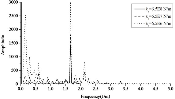
Fig. 11The frequency spectrum of contact force at speed of 200 km/h

Figs. 12, 13 shows the impact factors of rail deflection and wheel-rail force in case of three different slab bearing stiffness. When the slab bearing stiffness decrease, the rail deflection and wheel-rail force change acutely and show a trend of acceleration to a large degree. Obvious resonance peaks of rail deflection and wheel-rail force both appear. The lower the slab bearing stiffness is, the more obvious the peak impact response at the resonance speed is. If the slab bearing stiffness decrease and the speed increase, the frequency component caused by slab bending will be inspired, and the frequency component caused by rail pad spacing tends to be less, so the resonance peak doesn’t correspond to the theoretical prediction in Table 2. As a whole, the lower slab bearing stiffness will amplify dynamic response, change the wheel-rail force frequency component, and make the prediction of rail resonance more difficult.

Fig. 12Increase of impact factor of rail deflection at different slab bearing stiffness

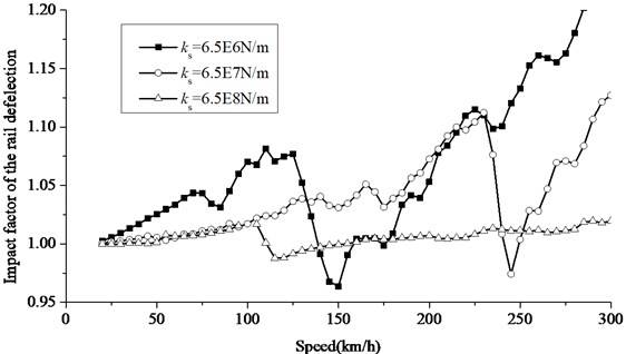
Fig. 13Increase of impact factor of contact force at different slab bearing stiffness

5.3. Comparison with vehicle and sprung mass

A comparison between the dynamic responses caused by a vehicle and a sprung mass traveling on the slab track is done. The slab bearing stiffness is $k_s=$6.5×10⁸ N/m, and the rail pad stiffness is $k_p=$6×10⁷ N/m.

Figs. 14, 15 shows the impact factors of rail deflection and wheel-rail force calculated by different models. It can be seen that the changing trends are exactly the same. But the rail deflection impact tends to be more obvious at the resonance peak when a vehicle travel on the rail because of the continuous impact by the front and rear wheels.

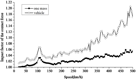
The wheel-rail force resonance peaks caused by a vehicle and a sprung mass traveling on the slab track both appear at the first-order resonance speed. But as a result of the car body pitch caused by the asynchrony of front and rear wheelsets, the wheel-rail force impact factor increases acutely when the speed increase.

Fig. 14Increase of impact factor of rail deflection based on different models

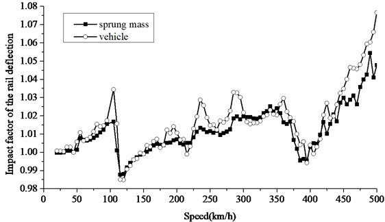
Fig. 15Increase of impact factor of contact force based on different models

6. Conclusions

In this study, the dynamic response of slab track under moving vehicle and sprung mass are investigated by means of finite element method. the wheel-rail resonance are investigated through theoretical derivations and numerical simulations. Several conclusions can be reached:

1) Vibration attenuation of slab track is low so the peak resonance is more easily induced. The higher the slab bearing stiffness is, the more obvious the response caused by rail pad spacing is. The resonance speed is about 100 km/h. If the track damping is too low, resonance will be much acute, and the wheel-rail wear and rail damage may worsen in practice.

2) To increase the rail pad stiffness will increase the resonance speed to a small degree and aggravate wheel-rail resonance response at the resonance speed.

3) With the slab bearing stiffness decrease and the speed increase, the wheel-rail force frequency components caused by slab deflection and vibration is easily inspired and there are several force frequency components. The resonance peaks tend to be more and more, and the impact factor of dynamic response at resonance speeds gets larger.

References

-
Zhu S., Cai C., Spanos P. D. A nonlinear and fractional derivative viscoelastic model for rail pads in the dynamic analysis of coupled vehicle-slab track systems. Journal of Sound and Vibration, Vol. 335, 2015, p. 304-320.
Zhai W., Wang K., Cai C. Fundamentals of vehicle-track coupled dynamics. Vehicle System Dynamics, Vol. 47, Issue 11, 2009, p. 1349-1376.
Kuo C., Huang C., Chen Y. Vibration characteristics of floating slab track. Journal of Sound and Vibration, Vol. 317, Issues 3-5, 2008, p. 1017-1034.
Steenbergen M. J. M. M., Metrikine A. V., Esveld C. Assessment of design parameters of a slab track railway system from a dynamic viewpoint. Journal of Sound and Vibration, Vol. 306, Issues 1-2, 2007, p. 361-371.
Yang L. A., Powrie W., Priest J. A. Dynamic stress analysis of a ballasted railway track bed during train passage. Journal of Geotechnical and Geoenvironmental Engineering, Vol. 135, Issue 5, 2009, p. 680-689.
Lou P. A vehicle-track-bridge interaction element considering vehicle's pitching effect. Finite Elements in Analysis and Design, Vol. 41, Issue 4, 2005, p. 397-427.
Luo Y., Yin H., Hua C. The dynamic response of railway ballast to the action of trains moving at different speeds. Proceedings of the Institution of Mechanical Engineers, Part F: Journal of Rail and Rapid Transit, Vol. 210, Issue 2, 1996, p. 95-101.
Dukkipati R. V., Dong R. Idealized steady state interaction between railway vehicle and track. Proceedings of the Institution of Mechanical Engineers, Part F: Journal of Rail and Rapid Transit, Vol. 213, Issue 1, 1999, p. 15-29.
Dong R. G., Sankar S., Dukkipati R. V. A finite element model of railway track and its application to the wheel flat problem. Proceedings of the Institution of Mechanical Engineers, Part F: Journal of Rail and Rapid Transit, Vol. 208, Issue 1, 1994, p. 61-72.
Cited by
About this article
This work was supported by the Fundamental Research Funds for the Central Universities (2014JBZ012).