Experiment and simulation research of the ground-borne vibration for a high-speed train

2.1. Establishment of wheel-track coupling model

In the operation system, the wheel-track system is a complex dynamic interaction [12]. Under the vibration loads, the periodical vibration loads will cause track vibration. The vibration on the contact point between the wheel and track is also caused by the load, and it also causes the elastic wheel-track deformation in the normal direction and creeping wheel-track slip change in tangential direction of the contact point. Besides, the wheel-track coupling vibration will be affected by the vibration of wheel-track force, thus affecting the system vibration. Therefore, a dynamic model for wheel-track coupling analysis needs to be established. The wheel-track coupling vibration can be divided into the vertical direction, horizontal direction and longitudinal direction [13]. The dynamic characteristics of the linear segment are mainly studied in this paper, and the vertical and horizontal effects are primarily considered. The coupling model diagram can be seen in Fig. 1.

According to the reference [2], the wheel-track coupling dynamic model is shown as below:

where $x$ is the operating train distance, $A$ is the coefficient matrix, $\upsilon$ is the train speed, and $t$ is the operating train time. $P_{c1}$ is the force between the first wheel-set and the track, while $P_{c2}$ is the force between the second wheel-set and the track. $m_w$ is the mass of the wheel-set. As known from nonlinear Herz contact theory [4], the wheel-track force is as follows:

where $\delta y\left(t\right)$ is the compressive modulus of elasticity between the wheel and track, and $G$ is the wheel-track contact parameter, which is related to the elastic modulus of wheel radius $R$, wheel and track material as well as the Poisson’s ratio. For cone-tread wheel, $G=4.75R^{-0.149}\times 10^{-8}$, and for worn-type wheel, $G=3.86R^{-0.115}\times 10^{-8}$.

The compressive modulus of elasticity between the wheel and track includes the hydrostatic pressure of the wheel, which can be directly determined by the displacement of the wheel and track at the wheel-track contact point, as shown below:

wherein, $y_{wi}\left(t\right)$ is the displacement of $i$th wheel at time $t$, and $y_r(x_{pi},t)$ is the displacement of the wheel under the $i$th-wheel displacement at time $t$. With displacement irregularity input of $y_0\left(t\right)$ in the wheel-track interface, the wheel-track force can be displayed as below:

wherein, $a$ is the depth of the irregularity, while $l$ means the length of the irregularity. The impact of track irregularity is primarily considered in the paper, and other secondary factors are thus ignored; it is regarded that the wheel and track are in consistent contact during the operation process of the train, where the track irregularity is represented by the continuously unsmooth harmonic. Two wheels of a bogie have different positions in the irregular track surface, so as the wheel-track force is also different. According to the fixed wheelbase of the bogie, the irregularities of the first and second wheel-sets are as follows:

wherein, $l_1$ is the irregular distance between the first wheel-set. The spectrum of the track irregularity is obtained from experiment, which can be substituted into the above equations so as to obtain the vibration acceleration under the wheel-track coupling.

Fig. 1Vertical and horizontal contact models between wheels and track

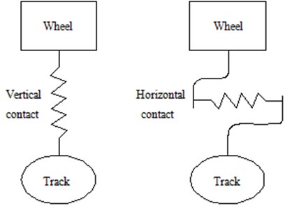
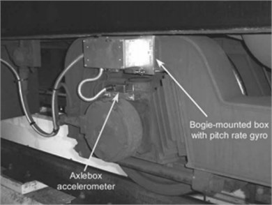
Fig. 2Track irregularity experiment

2.2. Impacts of different speeds

There are three dynamic performance indexes to evaluate the safety and comfort of a train, which is acceleration, limited value of wheel-rail force and rate of wheel load reduction. In the paper, the index of acceleration is focused [14].

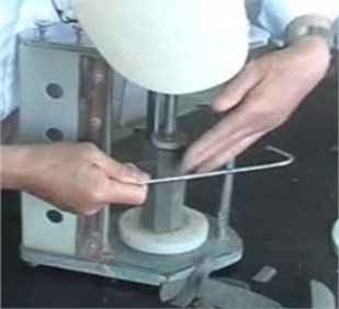
The track irregularity can be obtained from a bogie-mounted pitch-rate gyro. Sensors were mounted on the bogie, axle-boxes, as shown in Fig. 2. The spectrum of the irregularity of two wheel-sets can be obtained under the operating condition, whose results are shown in Fig. 3.

Fig. 3Spectrum of track irregularity of two wheel-sets

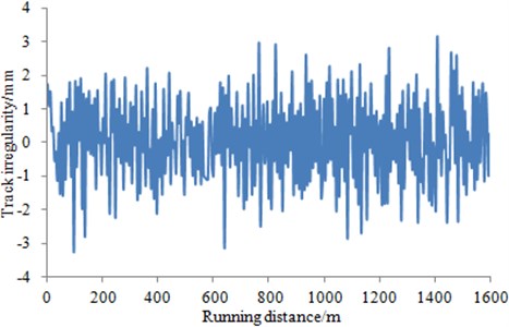
a) Spectrum of track irregularity of first wheel-set

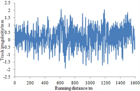
b) Spectrum of track irregularity of second wheel-set

The mass of the same train is fixed. Under the same condition, the impact of different train speeds is actually the impact of vibration frequency on the ground-borne [15]. The spectrum of the track irregularity obtained in the experiment is imported into the mentioned wheel-track coupling model of the train, so as to obtain the impact of the train speed on the acceleration, as shown in Fig. 4.

Fig. 4(a), (b) and (c) are corresponding to the acceleration-time relationship curves at the speed of 100 km/h, 200 km/h and 400 km/h, respectively. It can be obtained that the larger the train speed is, the greater the vertical acceleration and impact will be. And as the train mass is fixed under the same condition, the impact of the train speed on the train is also the impact of the vibration frequency on the train.

3.1. Test equipment

Fig. 5 is the dynamic triaxial equipment produced by UK GDS Company, which applies 5 Hz/10 kN/38-100 mm dynamic triaxial system (DYNTTS). The maximum diameter of the sample size is 300 mm, and the maximum confining pressure is 5 MPa. Therefore, the dynamic confining pressure test can be performed. In the vibration test, the soil body can be loaded with axial vibration force and set half-sine wave and other waves.

Fig. 4Vibration acceleration under different speed

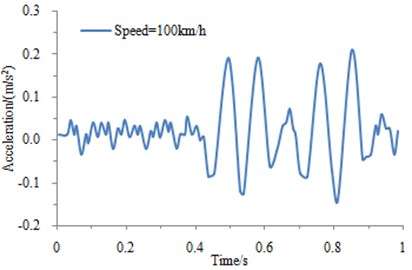
a) Speed = 100 km/h

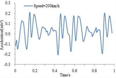
b) Speed = 200 km/h

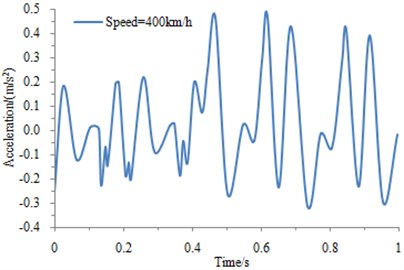
c) Speed = 400 km/h

3.2. Test process

Sample preparation: Soil is selected from an open space [16] near the high-speed train, and the soil is divided into silt and soft soil. The static pressure method is chosen to get the soft soil by mean of a thin-wall soil sampler. The sample preparation is made from the obtained undisturbed soil with the help of a cylinder with the cutting diameter of 3.8 cm and height of 8 cm [17].

Fig. 5Standard dynamic triaxial equipment

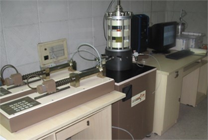
Fig. 6Sample preparation process

Experiment: The prepared soil sample is placed into an experimental instrument. The counter-pressure method is applied for saturation. And the reinforcement is set as 50 kPa, 100 kPa and 200 kPa, respectively.

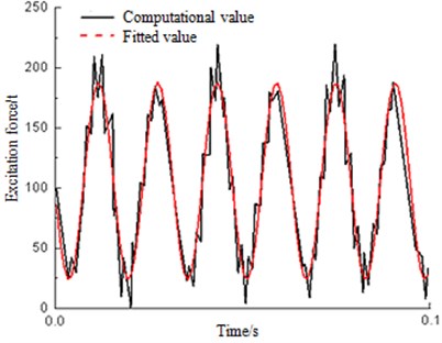
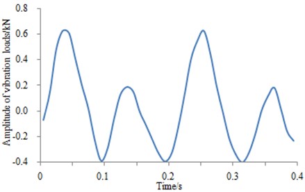
The calculation value of vibration load-time relationship curve is studied. Through computation, the vibration waveform changing with time can be acquired. A fitting can be further made and it can be found that the half-sine wave is most consistent with the vibration load-time relationship curve [18], as shown in Fig. 7. Fitting is conducted on the experimental curve, because the waveform of the actual vibration load is difficult simulated in the indoor test. As only sine waves are provided by the experimental instrument for loading, as a result, sine waves are thus applied in the paper for fitting. Therefore, it can be shown that in the indoor test of the high-speed train vibration load, although waveforms are not completely consistent, the minimum and maximum peak loads are basically accordant with very similar change. Among them, the fitting function is shown as Eq. (9), and parameters and standard deviations are shown as Table 1. It can be seen that the smaller the standard deviations are, the better the fitting effect will be:

wherein, $A>\text{0}$. Other parameters can be found in Table 1.

Fig. 7Calculation value and fitting value of excitation force

When vibration loads are added, the amplitude is implemented normalized process. The dynamic stress ratio is firstly defined as follows:

where ${\sigma }_d$ is the amplitude of dynamic stress. ${\sigma }_3$ is the confining pressure of the reinforcement. CSR is set to 0.1 and 0.2, and half-sine wave is selected as the vibration waveform. In order to analyze the effects of different frequencies, the vibration frequency is set to 0.25, 0.5, 1, 2.5, and 5 Hz, respectively, with the vibration number of 3,000 times.

3.3. Analysis of experimental results

By the indoor dynamic triaxial test, the vibration load of the high-speed train is simulated [19] to obtain that the dynamic strain-cycles relationship curve of different frequencies and dynamic stresses is a cluster of fluctuating curve, which is studied in many papers. MONISMITH has proposed an exponential strain curve as follows:

where $A$ and $b$ are parameters of the model determined by the least square method. $N$ is the number of vibration.

Meanwhile, Chai J. C. has made a normalized process for the stress amplitude and confining pressure as follows:

where ${\sigma }_d$ is the load amplitude, and ${\sigma }_s$ is the effective confining pressure. $a$ and $b$ are parameters of the model determined by the least square method. $N$ is the number of vibration.

A more classic relationship model between strain and the number of vibration is shown in Eq. (12), which has been verified by experiments since it had been proposed [11]. Such a model is applied since more comprehensive factors are considered in the model. Besides the soil, the influence factors of dynamic characteristics for soil include dynamic load amplitude, confining pressure, the number of vibration and vibration frequency. However, all the influence factors except the vibration frequency are taken into account in Eq. (12) proposed by Chai J. C. To describe the impacts of different train speeds, Eq. (12) was improved in the paper so that the impact of vibration frequency could be considered. Numerical value of the model parameters is shown in Table 2, which is determined by Eq. (12) based on the least square method.

In the experimental process, only the original soil structure is applied, and the GDS dynamic triaxial instrument is employed to change the vibration load amplitude, confining pressure, vibration frequency and the number of vibration. After obtaining the original experiment data, the model parameters in Eq. (12) and Table 2 are used for calculations. Finally, curves in Figs. 8-10 can be obtained.

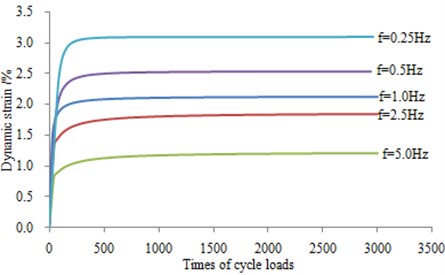
As can be seen from Fig. 8 to Fig. 10, the strain-cycles relationship curve is divided into three parts: The first stage is the rapid and elastic growth process. The second phase is the strengthened growth process, whose curve presents a slow increase and a turning point at this time. It is the elastoplastic stage. The third stage is the steady growth segment with a stable curve. With the increase of confining pressure, the stress amplitude is increased significantly. In addition, under the same confining pressure and different vibration frequencies, the strain value becomes smaller with the increasing frequency.

Fig. 8Stress-cycles relationship of different frequency under 50 kPa

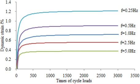
Fig. 9Stress-cycles relationship of different frequency under 100 kPa

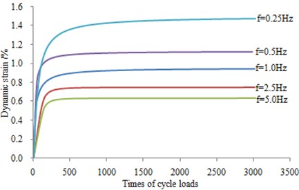
Fig. 10Stress-cycles relationship of different frequency under 200 kPa

3.4. Accumulative strain analysis with considering frequencies

The impact of frequency cannot be considered in Eq. (11). Based on CHAI J C’s formula, a strain-time model with considering frequencies is established as follows:

where ${\sigma }_d/{\sigma }_s=\text{0.2}$, $A_f$ is the functional expression of frequencies. $a$, $b$ and $m$ are selected with the following values 0.84, 0.13 and 2.0 by referring Table 3.

To establish a relationship between parameter $A_f$ and the frequency [20], the least square method is used to calculate, obtaining a relationship curve as shown in Fig. 11.

Fig. 11Parameter Af – frequencies relationship under different pressure

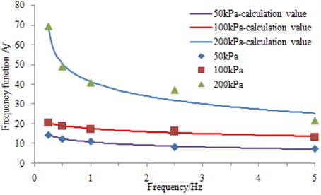
In the figure, ${\sigma }_s/{\sigma }_d=\text{0.2}$ is chosen for research. The curve is conducted for the calculation and analysis, thus acquiring a calculation formula of parameter $A_f$:

wherein, $f$ is the vibration frequency; $m$, $n$ and $l$ are calculating parameters of the formula, as shown in Table 4.

4.1. Establishment of high-speed train model

Targeting at a high-speed train project, a research is carried out in the paper. The tested road structure is the earth-filled embankment. And the geometrical dimensions of the model are as follows. The length of top ground-borne layer is 13.4 m, thickness of the ground-borne and embankment is 2.9 m, and the design slope gradient is 1:1.5, with the length of 25 m and depth of 15 m recommended according to the references [21]. Boundary conditions are as follows: the left and right displacement is constrained in $X$-direction, and the displacement in the bottom is fixed. The vibration load amplitude was set in the load modulus during the loading process, and the near sine load is selected. There are 1621 nodes and 2500 elements in the model. CPE4P four-node pore pressure element is applied as the element type of the model. And the plastic constitutive modules that come with the software are used as the material: namely the Mohr-Coulomb material model, which has been set in the Property modulus of ABAQUS software as shown below. The figure is not beautiful enough. In addition, considering the length of the paper, as a result, it is not included in the paper. The parameters have been chosen with the following values: cohesion $c=$11 kPa, internal friction angle $\phi =$9°, and dilatancy angle $\psi =$0°. The permeability coefficient would be $k=\mathrm{}$10^-9 m/s without a dilatancy phenomenon, the elastic modulus would be 207000 MPa, and the Poisson's ratio would be 0.3 [22].

In the analysis by means of experiments and theoretical calculations, the applied load is close to sine wave as shown in Fig. 7. Therefore, the load close to the sine wave should also be applied in the finite element model for more realistic simulation of this process. The load schematic diagram as shown in Fig. 12 is also presented by setting different parameters in ABAQUS software. For clear description, the corresponding control equations are also added in the paper. These parameters can be determined by Eq. (9) and Table 1 in the paper:

wherein, $A_0$, $A_n$, $B_n$ are constant values; $\omega$ is the circular frequency; $t$ is the vibration time and $t_0$ is the initial time.

Fig. 12Load vibration waveform added into finite element model

The acceleration vibration load is a uniform load with the amplitude of 30 kPa. In order to facilitate its comparison with the experimental part, the number of vibration is set to 10 million times.

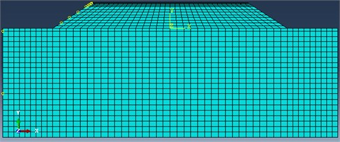
The CPE4P four-node pore pressure element is applied in the model. According to its stability condition, meshes are set under the Mesh module, and FEM of the ground-borne is established, as shown in Fig. 13.

Fig. 13Finite element model of the ground-borne

4.2. Comparative analysis of settlement value

After the initial verification, the model is submitted for the finite element calculation, and stress contour is obtained as shown in Fig. 14.

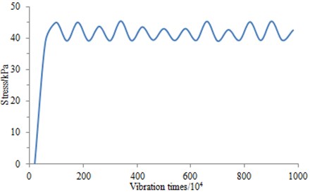
In consideration of the long operation for the current high-speed train, the ground-borne has been compacted densely under the long-term vibration loads [23]. Therefore, the initial vibration times in Fig. 13 are assumed to be 10 million times, and initial value of the long-term deformation is set to 0. That is to say, only vertical deformation produced from more than 10 million times of vibration loads is studied [24]. As can be seen from Fig. 16, the vertical deformation of ground-borne is occurred slowly with the increase of the vibration times, and the average vertical deformation is about 0.08 mm to 0.14 mm for every one million times. Its stress-times relationship is also shown in Fig. 15. As can be seen from Fig. 15, when the vibration times increases to one million, the stress change is close to sine curve, which is similar to the applied loads in Fig. 12. Fig. 12 is the load applied into the finite element model. As shown in the figure, the load is similar to a sine curve. When the load is just applied into the finite element model, with the increasing time of the applied load, the foundation will bear the increasing vibration times and stress, as shown in Fig. 15. However, the load applied into the foundation will decrease as time continues to go on. In the meanwhile, the foundation will bear gradually decreasing stress. In this case, the final stress curve is obtained and shown in Fig. 15. The foundation stress calculated by reference [25] is similar to the result of this paper. The above analysis proves that Fig. 15 is reliable.

Fig. 14Results of finite element simulation for the ground-borne

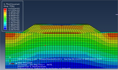
Fig. 15 is substituted into Eq. (13) established herein, and then the layering method is applied to calculate the final settlement. Finally, the calculation value is also compared with the experimental value, as shown in Fig. 16. As can be seen from the result, the experimental value is consistent with the calculated value. As a result, the improved formula is reliable.

Fig. 15Relationship curve between stress and vibration times for the ground-borne

4.3. Reinforcement measure and calculation analysis

Through the above mentioned calculation, it is found that the predicted value is closer to the experimental value, and the FEM of ground-borne can make accurate prediction and calculation. In order to control and prevent settlement, the reinforcement measurement is taken [26]. There are a lot of holes in the foundation as shown in Fig. 17. Then, the concrete is injected into the holes. The water-cement ration is 0.55 and density is about 1.62 g/cm³. In addition, 0.20 % citric acid solution is added, and the temperature is maintained at 29 C°, finding that the initial setting time of the slurry is 1.65 hours, and calculi rate of slurry solution is 96 %. The flow rate of the injected slurry reaches 12 L/min. The single injection of the slurry solution is 150 L and 225 L, respectively [27-29]. Finally, the corresponding computation results can be obtained as shown in Fig. 18.

Fig. 16Settlement-vibration times curves of the ground-borne

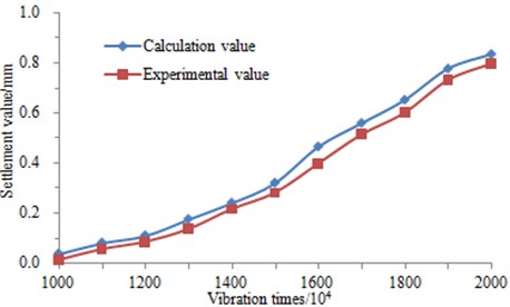
Fig. 17Schematic diagrams of reinforcement strategy

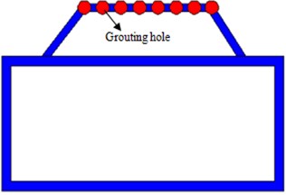
Fig. 18Results of finite element simulation for the ground-borne after reinforcement

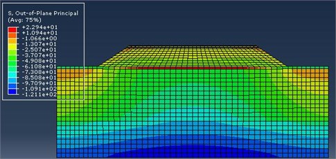
Fig. 19Relationship curve between stress and vibration times for ground-borne before and after reinforcement

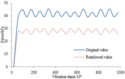
It is obtained from the finite element calculation that the stress value of the reinforced for the ground-borne is shown as Fig. 19, reaching 22.9 kPa in the maximum value. It is about half of maximum stress value before the reinforcement. The stress-times waveforms before and after reinforcement is similar.

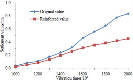
Similar to the above method, the finite element stress value of the reinforced ground-borne [30, 31] is substituted into Eq. (13), and layered method is applied to calculate the settlement value, as shown in Fig. 20. The settlement value is controlled obviously.

It can be obtained through the calculation and comparison that the reinforced ground-borne is reduced by half in terms of the final settlement. It thus indicates that the uneven settlement can be effectively controlled by the reinforcement measure. As a result, the impacts of long-term vibration on ground-borne can be prevented.

Fig. 20Settlement value of ground-borne before and after reinforcement