Dynamic response and limit analysis of buried high-pressure gas pipeline under blasting load based on the Hamilton principle

1. Introduction

In dynamic problems, the classical variational principle is the Hamilton principle [1]; it plays an important and fundamental role in the derivation of dynamic equations, the establishment of the finite element model and some other theoretical aspects. In the Hamilton principle, it is stipulated that in a specified system, the integral of the sum of the first-order variation of kinetic energy, the first-order variation of potential energy and the first-order variation of the work of the external force should be zero at any time interval $t_1$ and $t_2$ [2]. For the non-conservative system of elastic-plastic material, there will be energy dissipation in the structural system. In this study, the energy dissipation was introduced into the Lagrange function and a dynamic control equation was established for a non-conservative system consisting of elastic-plastic material according to the Hamilton principle. Because explosion impact load is the main load form of damages leading to oil and gas pipeline failure, it is of great significance for pipeline safety and protection to study the response characteristics and laws under the impact of an explosion of a buried high pressure natural gas pipeline. The numerical simulation models for a buried structure under explosion load effect mainly include the semi-empirical method, high explosive materials model (e.g., Arbitrary Lagrange Eulerian algorithm, ALE) [3], and method of empirical pressure time history on the explosion cavity inner wall [4]. These common empirical equations are basically based on statistical analysis of the amount of experimental results, obtained via the dimensional analysis method. For explosion shock problems, there will be a large error in empirical equations due to large discreteness of the measured values [5]. Commercial finite element software LS-DYNA can provide the high explosive material model and state equations for all types of explosives, accurately simulate the spread of the shock wave and structure dynamic response, present good simulation results among various types of explosive values, and yet will take a long time to calculate using the ALE method. The empirical stress time history method can avoid the simulation of the blasting cavity forming process and reduce the computational cost and the calculation error, which can meet the engineering needs [5]. In terms of the resistance to explosion of lifeline projects such as buried pipelines, the safety distances have been investigated when pipes were subjected to blast loads [6-9]. Kanaraehos et al. [10] proposed a new evolutionary model to calculate the peak speed, the model can be used in simplified calculation for a buried natural gas pipeline when near an explosion. Provatidis et al. [11] studied the strain analysis method for a buried pipeline under explosion impact load. Lagasco et al. [12] studied the influence of explosion tunneling on an adjacent buried pipeline and proposed a design chart related to distance from the explosive source, media, the backfill layer and pipeline material characteristics. Recently, Zhang et al. [13], Ji et al. [14], Wang et al. [15] and Mokhtari et al. [16] carried out a parametric study on the response of buried steel pipelines with plastic deformation during intentional explosions. In this article, a time history method of directly pressuring the charging cavity was used to calculate the blasting cavity radius, and specific parameters of pressure time history were obtained according to the U.S. army technical manuals TM5-855-1[17]. Then, a finite element model of interaction among blasting cavity-soil medium-high-pressure natural gas pipelines was established based on LS-DYNA finite element software; the dynamic response of a buried high pressure natural gas pipeline was detected. Finally, the critical explosive load, distance from the explosive source and wall thickness of a buried natural gas pipeline under explosion impact could be identified according to three types of limit load methods, during which explosive payload, distance from the explosive source and pipeline wall thickness were taken as generalized loads. Therefore, the calculating method and related results in this research can provide a certain reference basis for practical engineering pipeline safety operation and blasting construction schemes.

2. Elastic-plastic dynamic control equation based on Hamilton principle

The dynamic finite element program is based on the dynamic control equation [18]. Here, the energy dissipation was introduced into the Lagrange function and the finite element format of the elastic-plastic body dynamic control equation was derived, considering energy dissipation, according to the Hamilton principle. As we known, the energy dissipation was existed in most of the structural systems, Reyes-Salazar et al. [19, 20] did some analytically studied of energy dissipation of the steel frames with partially restrained connections subjected to seismic loading. Zhou et al. [21] designed a full-scale test to describe the damping of stay cable with passive-on magnetorheological dampers.

Here, firstly, for a unit cell, assume that the kinetic energy of an element is $T$, strain energy is $U$, and external potential energy is $W_e$. For a conservative system, the Lagrange function can be written as follows [2]:

For a non-conservative system consisting of an elastic-plastic medium, assume that the plastic dissipation power is $W_d$; the Lagrange function can be established as:

Set $u$ as a displacement vector of any point in a unit body and $u^e$ as a displacement vector of each node, which is a function of time $t$. Let the displacement vector of any point in the element $u$ be expressed by the displacement vector of each node $u^e$ as:

where $N$ is a shape function matrix, which is a function of coordinates $x$, $y$, and $z$:

Thus, the kinetic energy of an element can be obtained as:

where $\rho$is the mass of the element.

According to geometric considerations, the relationship between strain and the nodal displacement should be:

where B is the strain displacement matrix, which is a geometric matrix, independent of time $t$.

Thus, the relationship between strain rate and node rate should be:

and the strain energy for an elastic-plastic medium element should be expressed as:

where $\stackrel{-}{U}$ represents the strain energy of the unit cell.

There will be damping in every actual structure, and the damping will greatly affect the structure dynamic response amplitude and phase when calculating the structure dynamic response under a dynamic load; therefore, it is extremely important to correctly describe the analysis of structure dynamic response from structural damping. The damping dissipation of the structure can be divided into two parts: (1) dissipation related to the mass point moving speed, whose dissipation force is proportional to the mass point moving speed; (2) dissipation related to the strain rate.

For the first part of damping dissipation, assume that the damping coefficient is $c$ when the unit body vibrates; thus, the damping force on the unit body $f_v$ is:

For the second part of damping dissipation, the generalized damping force $f_r$ related to the strain rate is given by:

where $D$ represents the elastic matrix and $\beta$ is a constant.

Thus, the dissipated energy of the damping force on the unit body is:

The external force on the unit body can be divided into two parts: volume force $f=\left(f_x,f_y,f_z\right)$ and surface force $\stackrel{-}{t}=({\stackrel{-}{t}}_x,{\stackrel{-}{t}}_y,{\stackrel{-}{t}}_z)\text{;}$ the corresponding potential energies are $W_{e1}$, and $W_{e2}$, respectively, which are estimated as:

Thus, the Lagrange function is:

According to the Hamilton principle [22-25], integrating L over time interval ($t_1$, $t_2$) and letting the variation be equal to 0 yield:

The variation of each item in the Lagrange function can be expressed as follows:

Substituting Eq. (17)-(23) into Eq. (16) and taking the subsection integral, considering $\delta u^e\left(t_1\right)=0$, $\delta u^e\left(t_2\right)=$0, the following equation is obtained:

Let $K^e$, $M^e$, $C^e$, $F_q$, $F_p$ represent the stiffness matrix, mass matrix, damping matrix, external load matrix and generalized load matrix produced by plastic deformation of the unit body, respectively; then:

Therefore:

Because the integral interval is not specified, the integrand is given by:

Because the variation of unit body $\delta {\left(u^e\right)}^T$ is not specified either, it yields:

That is:

Rewriting Eq. (29) in an incremental form of the dynamic control equation yields:

In Eq. (30), $\mathrm{\Delta }{F}_{ext}$ and $\mathrm{\Delta }{F}_p$ represent the matrix incremental of the external load and the generalized load matrix incremental produced by plastic deformation, respectively; the expressions are: $\mathrm{\Delta }{F}_p=\underset{v}{\iiint }{B}^{T}D\mathrm{\Delta }{\epsilon }_{p}dV$, $\mathrm{\Delta }{F}_{ext}=\underset{v}{\iiint }{N}^T\mathrm{\Delta }fdV+\underset{S}{\iint }{N}^T\mathrm{\Delta }\stackrel{-}{t}dS$.

The dynamic finite element program can solve the dynamic equations via a time integral step by step; thus, it requires selection of a suitable loading time step to control the stability of the solution. If the loading time step $\mathrm{\Delta }t$ is too small, the calculation time will be increased, while too large a loading time step $\mathrm{\Delta }t$ will affect the calculation accuracy. For a dynamic load such as an explosion and impact, the time step in this article is determined according to reference [25] as follows:

where $\mathrm{\Delta }l$ represents the feature size of the smallest unit in the structure and $\lambda$ represents the longitudinal wave velocity.

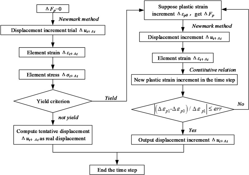
For a dynamic load such as an explosion and impact, the incremental form of dynamic control Eq. (30) can be solved by combining the Newmark method and plastic iteration; the specific process is briefly shown in Fig. 1.

Fig. 1Flow chart for solving the governing equations of elastic and plastic dynamics

3. The shape and loading mode of an explosion load

3.1. Determination of explosion load

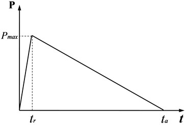
When an explosive buried in a soil medium explodes, enormous energy will be released instantaneously and the soil medium will form an explosion cavity due to the radial motion from the extrusion of the explosion products. The loading method of an explosion load in numerical simulation is different. The loading mode mentioned in references [26-30] was adopted in this project to add radial pressure on the explosion cavity wall formed after explosion; we consider the medium broken zone outside the explosion cavity as the elastic-plastic zone. It is very important to simplify the explosion load because different forms of load can form different stress fields. A large number of experiments and analyses show that using a triangle function can well describe the present good reliability of the explosive stress field of surrounding media. Therefore, the explosion load wave shown in Fig. 2 was adopted in this article, where $P_{max}$ is the maximum overpressure, $t_r$ is pressure rising time, and $t_a$ is positive pressure duration.

According to the U.S. army technical manuals (TM5-855-1), the pressure rising time $t_r=0.1t_a$ and the load arriving time $t_a$ are related to propagation distance and to the longitudinal wave velocity. The peak pressure could be calculated as [17]:

32

$P_{\mathrm{m}\mathrm{a}\mathrm{x}}=48.77\gamma \left(\rho c\right){\left(\frac{2.78R}{W^{\frac{1}{3}}}\right)}^{-n}.$

In Eq. (32), $\rho c$ refers to rock and soil medium wave impedance; $R$ refers to the distance from the explosion point; $W$ is the explosive weight; $n$ is the site attenuation coefficient; $\gamma$ is the explosive coupling coefficient; for underground closed explosion, $\gamma =$1.0.

Fig. 2Pressure time history of explosion cavity internal wall

4. Simulation model and parameters

4.1. Simulation model

The outer diameter of the buried high pressure natural gas transmission pipeline is $D=$1016 mm; the inner gas pressure is $P=$10 MPa. Based on the LS-DYNA Theoretical Manual, SOLID164 was selected as the three-dimensional discrete element of the soil and pipe in the explicit dynamic finite element analysis process, during which the multi-material ALE algorithm was embedded in every solid element. The explosion simulation was established by exerting radius pressure on the inner wall of the explosion cavity based on the empirical relationship. A finite element model for interaction among the explosion cavity, rock and soil medium, and natural gas transmission pipeline could then be built based on the calculation of the explosion radius according to the quasi static theory. Because the calculation was based on the empirical pressure time history method exerted on the inner wall of the explosion cavity, the actual pressure on the inner explosion cavity wall should be much smaller than that of the explosion center; thus, the calculation stability could be guaranteed by adopting the Lagrange element. In total, there were 21510 elements in the finite element model for the pipeline and soil, where 600 elements were for the pipeline and 20910 elements were for the soil in total; the total node number was 24492, as shown in Fig. 3. The calculation working conditions are listed in Table 1.

Fig. 3Finite element model

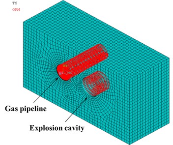
Table 1Working conditions for calculation

Case	Working condition	Explosive payload $W$ / kg	Distance from explosion point $R$ / m	Pipeline wall thickness $T$ / mm	Transmission pressure / MPa
No. 1	1	1.25	2	14.6	10
	2	2.5	2	14.6	10
	3	7.5	2	14.6	10
	4	10	2	14.6	10
	5	12.5	2	14.6	10
No. 2	1	12.5	2	14.6	10
	2	12.5	2.5	14.6	10
	3	12.5	3	14.6	10
	4	12.5	4.5	14.6	10
	5	12.5	8	14.6	10
No. 3	1	12.5	2	14.6	10
	2	12.5	2	17.5	10
	3	12.5	2	21	10
	4	12.5	2	26.2	10
	5	12.5	2	28	10

5. Dynamic response of buried high pressure natural gas transmission pipeline under explosive load

The explosion cavity radius and pressure time history can be calculated by using the empirical pressure cavity wall method, as well as the shock wave propagation in soil formed by the explosion, which can be clearly seen in Fig. 4(a). The simulation results show that the shock wave is almost uniformly spread around and that the pressure on the soil near the wave front edge area tends to be higher. As shown in Fig. 4(b), the observed drum package phenomenon of soil under an explosion can be modeled by using the explosion cavity theory. Take the 5th working condition of case 1 in Table 1 as an example; the pressure time history curves of three elements along the detonation wave propagation direction, from near to distant, named 20200, 16135, and 16735, are selected for calculation, as shown in Fig. 5. The results show that the pressure on the soil body increases sharply to its peak value and then declines rapidly. The peak pressure of element 20200, which is nearest to the explosion source, arises earliest and its peak value is the largest. The pressure time history curve of the soil body reflects the transmission characteristics of the detonation wave in the soil medium reasonably.

Fig. 4Finite element simulation of underground explosion

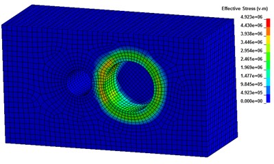
a) Shock wave propagation in soil body

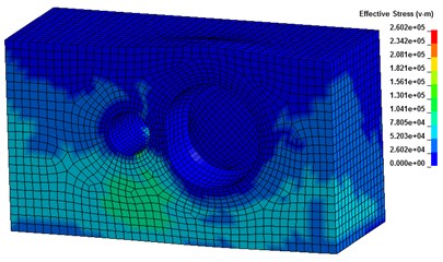
b) Bulge phenomenon of soil under explosion

Fig. 5Pressure time history curve for different soil unit bodies

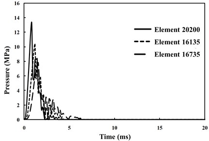
Fig. 6Equivalent stress time history curve under different explosive charges

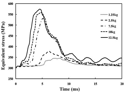
The hot point equivalent stress time history curve of the buried high pressure natural gas transmission pipeline is calculated from working conditions case 1, case 2 and case 3 in Fig. 6, Fig. 7 and Fig. 8. As shown in Fig. 6, the hot point equivalent stress time history presents the same variation tendency under different explosive payloads, but the more the explosive payloads applied, the larger the peak hot point strain value will be and the earlier the peak value will show up. Keeping the other parameters the same, the explosive cavity is dependent upon the explosive payload. Thus, when the explosive payload becomes larger, the radius of the explosive cavity will also be larger and the distance from the explosion load to the pipeline will be reduced; hence, the peak value of the hot point equivalent stress will arise earlier. It can also be determined that the peak value can only last for a very short time, generally a few milliseconds. The attenuation speed of the hot point equivalent stress peak value will increase with the increase of the explosive payload.

It can be seen from Fig. 7 that the variation tendency of hot point equivalent stress time histories is the same. As the distance from the explosion center increases, the hot point equivalent stress peak value will appear later and the stress peak value will decrease dramatically; when the distance from the explosion center decreases, the attenuation speed after the peak value will increase. Therefore, Fig. 7 can reflect the attenuation characteristics of the explosion shock wave with the increase of propagation distance.

Fig. 8 shows that near the 0 time point, with the increase of wall thickness, the initial hot point equivalent stress of pipeline steel will be smaller; under this working condition, the initial equivalent stress for a pipeline wall thickness of 28 mm will be almost half the value of the pipeline wall thickness of 14.6 mm. The peak values appear at almost the same time, while the peak value of the dynamic stress response is not sensitive to the change of the pipeline wall thickness. Under an explosion load, the variation tendencies of the hot point equivalent stress for pipelines with different wall thicknesses over time are almost the same; finally, the stress will fall back to the initial equivalent stress value.

Fig. 7Equivalent stress time history curve for different distances from explosion point

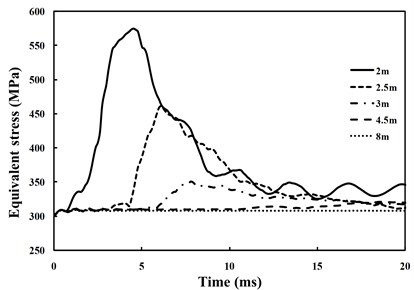
Fig. 8Equivalent stress time history curve for different pipeline wall thicknesses

6. Relationship between peak particle vibration velocity and explosion distance and payload

Because the effective parameter needed to measure the explosion vibration strength is particle vibration velocity, the quality of the numerical simulation will greatly affect the results of the particle vibration velocity. In engineering practice, Sodev’s empirical formula is often used to determine the vibration velocity of particles during blasting [36]:

where $v_{max}$ refers to the peak particle vibration velocity; $K$ is a coefficient related to the explosion field condition; $W$ is the explosive payload; $R$ is the distance from the measuring point and explosion center; $n$ is the attenuation coefficient.

The peak vibration velocities that correspond to an explosive payload of 1.25 kg, 2.5 kg, 7.5 kg, 10 kg and 12.5 kg are 2.68 m/s, 4.29 m/s, 7.07 m/s, 14.5 m/s, and 17.2 m/s, respectively. Using the least squares fitting method on Eq. (37), an expression Eq. (38) can be obtained; the fitting curve is shown in Fig. 9:

The coefficient $K$ related to the explosion field conditions should be 11.936 and the attenuation coefficient $n$ should be 2.5011 by comparing Eqs. (37) and (38). Observed from Fig. 9, with the increase of explosive payload $W$, the peak velocity of pipeline particles $v_{max}$ will increase gradually, and the relationship between $v_{max}$ and $W$ is almost linear.

Fig. 9Relationship between peak value of vibration velocity of particles and explosive payload

Fig. 10Relationship between peak value of vibration velocity of particles and distance from explosion center

The peak vibration velocities of pipeline steel that correspond to a distance from the explosion center of 2 m, 2.5 m, 3 m, 4.5 m, and 8 m are 17.21 m/s, 7.20 m/s, 3.02 m/s, 0.82 m/s, and 0.06 m/s, respectively. Using the least squares fitting method on Eq. (37), an expression equation such as Eq. (39) can be obtained; the fitting curve is shown in Fig. 10:

The coefficient $K$ related to the explosion field conditions should be 9.438085 and the attenuation coefficient $n$ should be 4.04711 by comparing Eq. (37) and (39). Observed from Fig. 10, with the increase of distance from the explosion center, the peak value of the particle velocity attenuates soon initially, and when the distance from the explosion center reaches a certain value, the peak velocity is stabilized and finally drops close to 0.

7. Limit analysis of buried high pressure natural gas transmission pipeline

For high grade pipeline steel, the common failure mode is the plastic defect. The plastic limit load of the elastic-plastic structure is the characterization of the maximum bearing capacity of the structure; therefore, if the structure is designed based on the plastic capacity, it will not only be beneficial for determining the plastic properties of the material but can also help to obtain the real safety margin of the structure [37]. Thus, the plastic limit load has become an important parameter for determining the pipeline pressure bearing capacity and the integrity of the structure. Under a theoretical limit load, the deformation of the structure will increase unlimitedly; then, the structure may lose the load bearing capacity consequently, during which an ideal elastic-plastic material with small deformation is assumed. In reality, strain hardening and the strain rate effect exist for the actual materials and the deformation is not a small one; thus, the theoretical state will not happen at all. Under actual operation conditions, after material goes into the plastic deformation stage, the relationship between stress and strain will present strong nonlinear characteristics. During the solution process, a complex mathematic problem will be encountered during calculation due to the material nonlinear constitutive relation, resulting in low calculation efficiency. To avoid the calculation difficulties resulting from the plastic deformation, the limit analysis method is widely used in the engineering field to determine the critical load. For an actual structure, the load when obvious plastic flow appears is often defined as the engineering limit load. Because there are different criteria for judging obvious plastic flow, different definitions for limit load are created. Three commonly used limit analysis methods are listed as follows:

7.3. Zero curvature criterion

This criterion is an improvement based on the tangent intersection criterion [39], as shown in Fig. 11(c). In this method, the way to determine the limit load is to draw the tangent of plastic flow in the load-strain curve; the limit load $P_{lc}$ is then defined as the load value of the separation point of the load-strain curve and the tangent of the plastic section.

The pipeline maximum strain was calculated under different explosive payloads, distances from the explosion center and pipeline wall thicknesses, according to the three cases shown in Table 1; the results are listed in Table 5, 6 and 7, respectively. The explosive payload, distance from the explosion center and pipeline wall thickness could be considered as generalized loads. The explosive payload in Table 5 was considered as variable from 1.25 kg to 12.5 kg; then, the corresponding strain magnitudes were calculated, as well as the pipeline deformation under different distances from the explosion center and wall thicknesses, as shown in Table 6 and Table 7. Therefore, the critical explosive payload, distance from the explosion center and pipeline wall thickness could be obtained according to the rule of solution methods to limit the load, as shown in Fig. 12, 13 and 14. For the limit values shown in Table 8, the explosive payload limit based on the tangent intersection criterion is more conservative than others, while compared to the other two limit analysis criterions, the zero curvature criterion may get relatively smaller limit prediction values with changing explosion distance or wall thickness.

Fig. 11Three common ultimate load rules

a) Tangent intersection criterion

b) Twice elastic slope criterion

c) Zero curvature criterion

Table 5Total pipeline strain under different explosive payloads

Buried pipeline with steel of X70; pipeline diameter of 1016 mm; gas pressure of 10 MPa; wall thickness of 14.6 mm; distance from explosion center of 2 m
Explosive payload $W$ / kg	1.25	2.5	7.5	10	12.5
Total strain $\epsilon$ / 10-3	1.400	1.535	2.190	3.170	4.498

Table 6Total pipeline strain under different distances from the explosion center

Buried pipeline with steel of X70; pipeline diameter of 1016 mm; gas pressure of 10 MPa; wall thickness of 14.6 mm; explosive payload of 12.5 kg
Distance from explosion center $L$ / m	2	2.5	3	4.5	8
Total strain $\epsilon$ / 10-3	4.498	1.901	1.444	1.332	1.273

Table 7Total pipeline strain under different pipeline wall thicknesses

Buried pipeline with steel of X70; pipeline diameter of 1016 mm; gas pressure of 10 MPa; explosive payload of 12.5 kg; distance from explosion center of 2 m
Pipeline wall thickness $T$ / mm	14.6	17.5	21	26.2	28
Total strain $\epsilon$ / 10-3	4.498	3.294	2.454	2.031	1.952

Fig. 12Three limit analysis methods to determine the explosive payload

Fig. 13Three limit analysis methods to determine distance from the explosion center

Fig. 14Three limit analysis methods to determine pipeline wall thickness

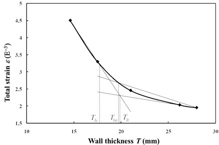
Table 8Results from different limit analysis criteria

Limit analysis criterion	Tangent intersection criterion	Twice elastic slope criterion	Zero curvature criterion
Explosive payload $W$ / kg	$W_{lt}=$8.12	$W_{l\phi }=$10.5	$W_{lc}=$9.21
Distance from explosion center $R$ / m	$R_{lt}=$2.51	$R_{l\phi }=$3.14	$R_{lc}=$2.33
Pipeline wall thickness $T$ / mm	$T_{lc}=$19.9	$T_{lc}=$19.7	$T_{lc}=$17.7

8. Conclusions

1) The dissipation energy resulting from particles’ moving velocity and the strain rate effect was introduced into the Lagrange function, a finite element format of the dynamics control equation was established for a non-conservative system consisting of elastic-plastic material, which could provide a basis for the calculation of elastic-plastic dynamic problems, and then a solution scheme for the control equation was proposed, with a method combining the Newmark method and plastic iteration.

2) In this article, a loading method for exerting pressure time history to the inner wall of the cavity formed by an explosion was adopted to establish a model of the dynamic interaction among explosion cavity-soil medium-high pressure natural gas transmission pipeline to simulate the propagation characteristics of the explosion shock wave in a soil body and the dynamic response characteristics of a buried high pressure natural gas transmission pipeline. The simulation results well reflect basic explosion phenomena and the dynamic response of the pipeline.

3) The dynamic response laws of hot point elements of a buried high pressure natural gas transmission pipeline were calculated and analyzed by setting different cases of working conditions under different explosive payloads, distances from the explosion center and pipeline wall thicknesses, and the relationship between maximum particle vibration velocity in pipeline steel and distance from the explosion center was fitted out using Sodev’s empirical formula. The results of this article could provide certain reference value for the construction, design and safety supervision of buried high pressure natural gas transmission pipelines and would also be beneficial for the development of the quantification and accuracy of pipeline risk assessment technology.

4) Considering the explosive payload, distance from the explosion center and pipeline wall thickness as generalized loads, the critical explosive payload, distance from the explosion center and pipeline wall thickness were determined for a buried high pressure natural gas transmission pipeline under the explosion shock effect based on three limit analysis criteria. The calculation methods and final results of this research could provide some references for the safe operation and blasting construction scheme of practical engineering pipelines.