Study of measured indoor low-frequency noise levels resulting from outdoor noise sources, using a simplified physical model as well as empirical and FEM calculations

1. Introduction

With the development of newer economic activities and the resulting increase in environmental noise pollution, it becomes increasingly important and relevant to predict the indoor noise level in newly-constructed buildings. To assess indoor noise levels coming from the outdoors, formulas found in architect-orientated manuals or textbooks, e.g.: [1-3] or the ISO 12354-3 [4] standard, are used, which are based on evaluation of the apparent sound reduction index (transmission loss) of the building façade (derived from the acoustic characteristics of individual façade elements) and include corrections according to the noise source (spectrum), the incident sound wave angle, the volume of the enclosed space or the sound absorption properties of the enclosed space’s walls. The formulas rely on average sound pressure levels (SPL) (indoors and outdoors) and equivalent SPL (if the sound levels change over time) and are adapted for predicting sound levels, presuming that a diffuse acoustic field is formed indoors. It means that the formulas do not take into account the possible forming of a standing wave effect, which appears at low frequencies and directly depends on the dimensions of the enclosed space.

The first aim of the study was to evaluate the distribution (spatial variation) of measured equivalent sound pressure levels and to compare them with calculated equivalent average sound pressure levels in the model. The second aim was to identify the possibility of using formulas specified in standard ISO 12354-3 for calculation of the indoor average sound pressure level at low frequencies from outdoor noise. The third aim was to apply FEM calculations for evaluation of spatial SPL distribution at the model and to evaluate if an average of the sound pressure level calculated from measurements at points along every 5 cm of the physical model would correspond to the average sound pressure level if it were measured at every possible position.

The study was performed in a classical way for acoustic science - using a simplified physical model, which is exposed to speaker-generated raised frequencies. Due to the fact that in many countries, low-frequency noise is regulated at centre frequencies of 1/3 width octave bands according to average SPL values (including the assessment of the SPL in a corner of the enclosed space) [5], the study of acoustic field analysis was performed in 1/3 octave bands. For the investigation of room modes and resonant frequencies of walls, for FEM calculations analysis of discrete frequencies was used.

2. Physical model of the enclosed space

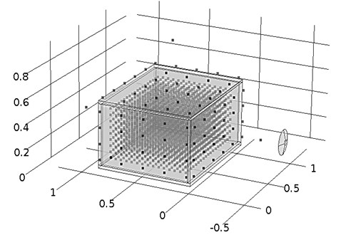
For the study, in order to model the low frequency (20-200 Hz) sound field behaviour in an enclosed space (room), a simplified (uniform) physical model was made and reduced in size by a factor of 5 (hereafter, “the model”), which was exposed to white noise at a frequency level 5 times higher (specified range of frequencies 10-1250 Hz). Before the analysis of the distribution of indoor equivalent sound pressure levels $L_{eq.\left(indr.\right)}$, the distribution of outdoor equivalent sound pressure levels $L_{eq.\left(outdr.\right)}$ was measured (see Figure 1).

The study was conducted in the Mechanical Vibration and Acoustic Noise Level Testing Laboratory of the Technological Systems Diagnostics Institute (Kaunas University of Technology). The acoustical hall of the laboratory has semi-anechoic properties (sound-absorbent walls and ceilings and a sound-reflecting floor). In order to reduce interference by sound waves around the model, a 50-mm-thick shield made of sound-absorbent glass wool panels Ecophon Industry Modus (manufacturer’s declared sound absorption coefficient $\alpha W=$ 1) was installed. The length of the shield: 3.6 m, width and height: 2.4 m. The top of the shield above the model was covered with a 2.4 m×2.4 m panel. The model was placed on a sound-reflecting (stone-tiled) floor.

The physical model is a box made from 25-mm-thick wooden chipboard. The inner dimensions of the model: length 1 m, width 0.8 m, height 0.5 m. The panel’s density (determined by weighing): 641.6 kg/m³. The manufacturer’s declared modulus of elasticity (Young’s modulus) $E=$2.5 GPa, Poisson's ratio 0.29. The sound reduction index of chipboard (which is measured in a noise suppression chamber at the Department of Environmental Protection of the Faculty of Environmental Engineering of Vilnius Gediminas Technical University, using standard ISO 16283-1) is from 12.5 dB to 39.1 dB in the frequency range of interest (see Table 3).

The acoustic field in the model was studied by applying white noise to the model. As a sound source, a loudspeaker (HQ POWER; Model: VDSG8 2-strip; FD diameter speaker (woofer size) 20 cm) was used. The loudspeaker was placed perpendicularly to the middle of the longest wall of the model at a distance of 60 cm. Such a small distance was selected to reduce standing waves that occur in the laboratory.

White noise generation and analysis is made using a Bruel & Kjear analyzer PULSE^TM and LabShop (Version 13.1.0) software. For amplifying the generated white noise, an MMF LV103 audio amplifier was used.

Due to the fact that low-frequency noise limit values are governed in 1/3 octave bands, the spatial equivalent sound pressure level variation inside the model was studied in 1/3 octave bands using CPB (Constant Percentage Bandwith) analysis. In a study “control” analysis of discrete (individual) frequencies at two horizontal cross-sections (5 cm and 25 cm-high), an analysis using FFT (Fast Fourier Transform) was also carried out.

To determine outside SPL, measurements of equivalent sound pressure levels $L_{eq.\left(outdr.\right)}$ were performed at a distance of 2 cm and 40 cm from all the external walls of model. When measuring 2 cm from the model façade, the microphone was directed perpendicular to the model. Measurements were taken every 20 cm in 4 rows. When measuring 40 cm from the centres of the model façades, the microphone was directed toward the sound source.

For acoustic field investigation inside the model $L_{eq.\left(indr.\right)}$, measurements were taken every 5 cm across the entire model space (at a total of 2,565 points), starting at 5 cm from the walls.

Fig. 1The model under study, with loudspeaker and SPL measurement points arranged inside and outside the model

3. Sound pressure levels outside the model

According to the ISO 12354-3 standard, to calculate the sound reduction index R' of building elements, the average (or the equivalent average) sound levels to an external surface of the building elements are needed. To calculate standardized or normalized level differences, the average sound pressure levels at a distance of 2 m from façades are needed. The measured equivalent sound pressure levels at a distance of 40 cm (corresponding to a distance of 2 m in a real situation) from the centres of the model façades as well as measured minimum and maximum equivalent sound pressure levels and calculated equivalent average sound pressure levels at a distance of 2 cm from the model façades are presented in Fig. 2.

The average equivalent sound pressure levels are calculated according to the following Eq. (1):

where $L_{eq1}$, $L_{eq2}$,…, $L_{eqn}$ measure equivalent pressure levels at positions 1, 2,..., $n$; $n$ – the number of measuring points.

Measurements of $L_{eq\left(outd.2cm\right)}$ showed that due to reflections of sound waves from the model façades and the floor and due to dimensions and properties of laboratory hall , non-uniform sound pressure affects the model façades and at different positions SPL at different bands varies: from 6.7 to 15.0 dB at the front façade, from 2.8 to 13.3 dB at the back façade, from 4.6 to 16.6 dB and from 4.3 to 17.3 dB respectively at the left and right façades, from 5.1 to 19.1 dB at the top façade.

Measurements show that the difference between $L_{eq\left(outd.40cm\right)}$ and $L_{eq\left(outd.2cm\right)}$ at distances of 2 cm and 40 cm from the model façades varies up to 9.1 dB.

Fig. 2Measured equivalent sound pressure levels Leqoutd.40cm at a distance of 40 cm (corresponding to a distance of 2 m in a real situation) from the centres of the model façades. As well as measured minimum and maximum equivalent sound pressure levels Leqoutd.2cmand calculated equivalent average sound pressure levels at a distance of 2 cm from the model façades

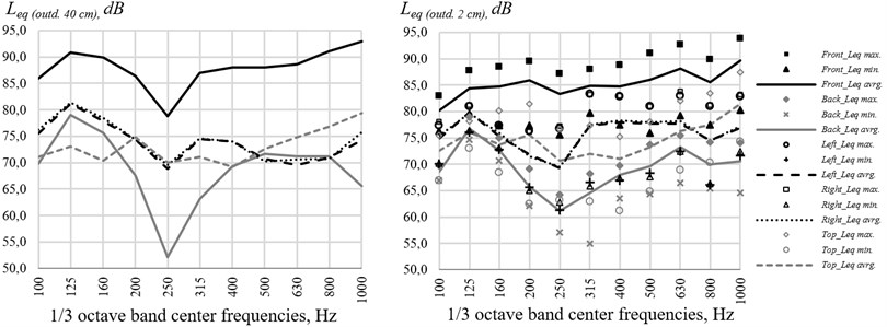
Fig. 3examples of measured Leqoutd.2cm: a) front façade at 250 Hz centre frequency 1/3 octave band; b) back façade at 250 Hz centre frequency 1/3 octave band; c) right façade at 400 Hz centre frequency 1/3 octave band; d) top façade at 630 Hz centre frequency 1/3 octave band

a)

b)

c)

d)

Fig. 4The difference between Leqoutd.40cmand Leqoutd.2cm

4. Sound pressure levels inside the model

In many countries where low frequency noise is regulated, limit values and measuring points, at which generalized (average) sound pressure levels must be assessed, are specified. For example, in Lithuania according to the hygiene norm HN30: 2009 [8], measurements are made in accordance with standard ISO 1996-2 [9]. The standard specifies that the low frequency noise measurement points in a space (room) should be evenly spread out, at places where persons exposed to noise usually spend their time and at least in three positions (without specifying the exact height). At least one of these three points should be in a corner at a distance of 0.5 m from all surfaces bordering the space (room) (e.g. the top or bottom corner of the room). In other countries, for example, Sweden or Denmark the angular point is 0.5 m from the wall but at a height of 1.5 m, and the other points (at least 2) at a height of: 0.6 m, 1.2 m or 1.6 m in Sweden and 1-1.5 m in Denmark [10]. It is assumed that SPLs in the corners are higher than the average SPLs of the room [10].

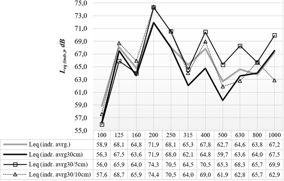
Fig. 5measured equivalent highest, lowest and calculated average sound pressure levels (Leqindr.max., Leqindr.min., Leqindr.avrg.at 1/3 octave bands inside the model compared to equivalent average sound pressure levels in the upper corners 5 cm and 10 cm from the walls (Leqindr.avrg45/5cm. andLeqindr.avrg40/10cm.) as well as to measured equivalent sound pressure levels and calculated equivalent average sound pressure levels at a distance of 2 cm from the front façade (Leqoutdr.max.2cm. andLeqoutdr.avrg.2cm.)

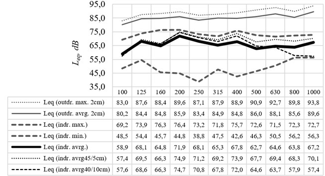
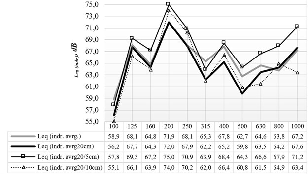
Fig. 6According to measurement results (at 1/3 octave bands), the calculatedequivalent average sound pressure levels at 20 cm height (Leqindr.avrg20cm.) compared to calculated equivalent average sound pressure levels in corners 5 cm and 10 cm from the walls at the same height (Leqindr.avrg20/5cm. andLeqindr.avrg20/10cm.) and compared to calculated equivalent average sound pressure levels in the entire model (Leqindr.avrg.)

After measurements inside the model (at 2,565 total positions), the equivalent highest, lowest and average sound pressure levels ($L_{eq\left(indr.max.\right)}$, $L_{eq\left(indr.min.\right)}$, $L_{eq\left(indr.avrg.\right)}$) throughout the model space were determined. Taking into account the norms of the various countries, the average sound pressure levels were calculated 20 and 30 cm above the floor (which corresponds to 1 m and 1.5 m in height in a real situation). In addition, the equivalent average sound pressure levels were calculated for the corners at a distance of 5 cm and 10 cm from the wall, and at a height of 20, 30, 40 and 45 cm ($L_{eq\left(indr.avrg.45/5cm\right)}\text{,}$$L_{eq(indr.avrg.40/10cm}\text{,}$$L_{eq\left(indr.avrg.20/5cm\right)}\text{,}$$L_{eq\left(indr.avrg.20/10cm\right)},L_{eq\left(indr.avrg.30/5cm\right)}$, $L_{eq(indr.avrg.30/10cm)}\text{.}$ The results are given in Figs. 5, 6 and 7.

Fig. 7According to measurements results (at 1/3 octave bands), the calculatedequivalent average sound pressure levels at a height of 30 cm (Leqindr.avrg30cm.) compared to calculated equivalent average sound pressure levels in corners 5 cm and 10 cm from the walls at the same height (Leqindr.avrg30/5cm. andLeqindr.avrg30/10cm.) and compared to calculated equivalent average sound pressure levels in the entire model (Leqindr.avrg.)

Spatial variation of measured equivalent sound pressure levels $L_{eq\left(indr.\right)}$ inside the model are presented below in Fig. 8.

According to theory (e.g.: [11], [12]), the highest sound pressure level differences indoors occur at the resonance frequencies of a room, so-called room modes. Resonance frequencies of a rectangular room with dimensions L, W and H can be calculated using the following Eq. (2):

where $p$, $q$ and $r$ are integers 0, 1, 2, 3,….

$c$ – speed of sound in air calculated using Eq. (3) [13]:

where $T$ – temperature °C.

Calculated room (model) modes at 23°C temperature are presented in the following Table 1.

Below the lowest room mode (at frequencies, that has a wavelength more than twice longer than room length) if building (or in our case physical model) construction acts as rigid body, sound pressure levels changes as in static air pressure. If resonant frequencies of walls or some construction elements exists, bigger SPL differences and different spatial distribution of SPL can be met. Resonant frequencies of walls can be calculated according to Eq. (4) [15]:

where $m$ and $n$ are integers 1, 2, 3; $a$ and $b$ are inner dimensions of wall; $h$ – thick of wall, $\rho$ – density of wall material; $E$ and $\sigma$ are the Young’s modulus and Poisson’s ratio respectively.

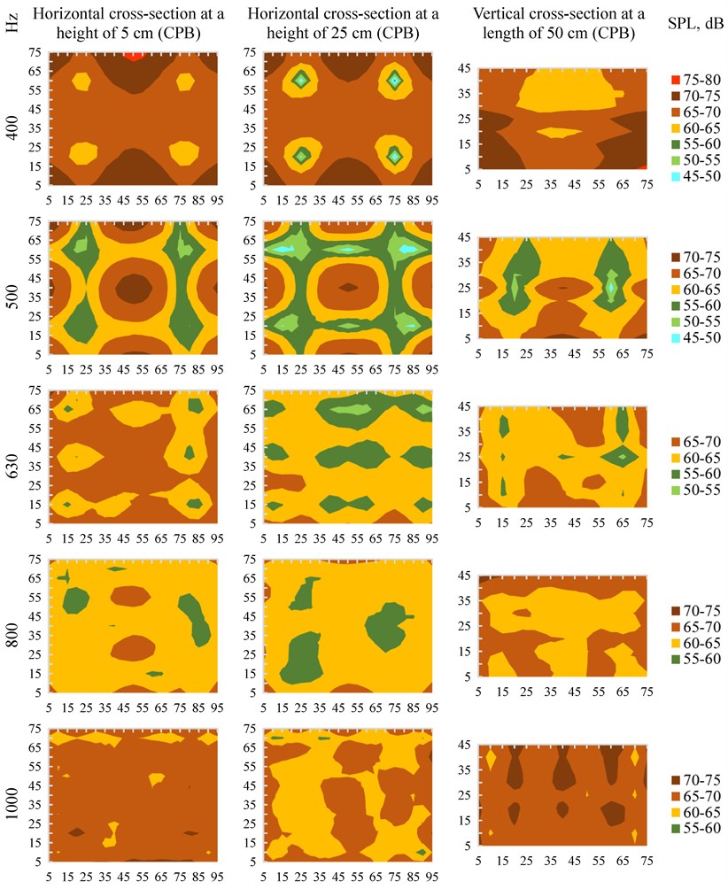
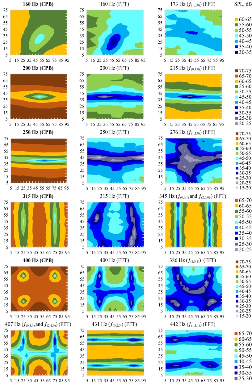
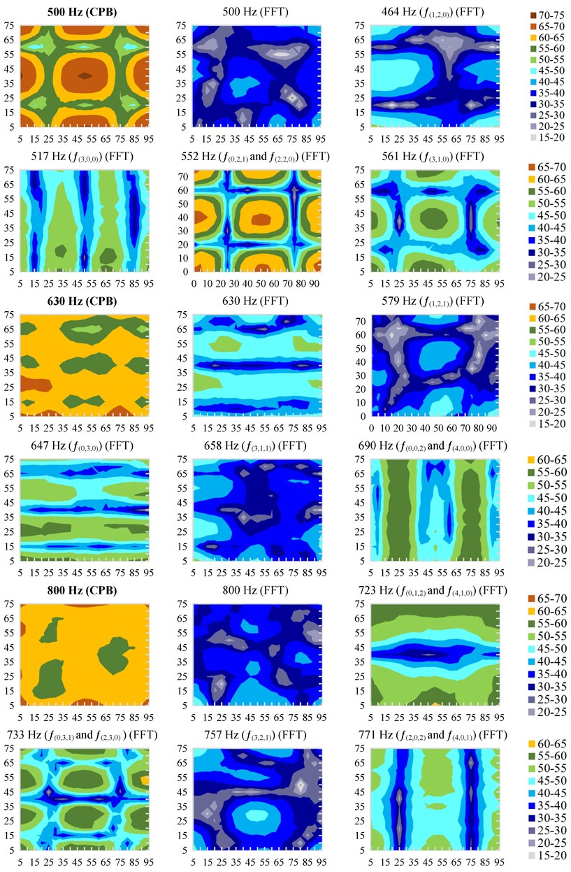
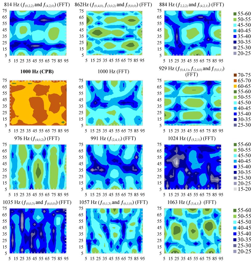
Fig. 8Cross-sections of spatial variation of measured equivalent sound pressure levels Leqindr. at 1/3 octave bands inside the model. Note: sound radiation direction is from the bottom of horizontal cross-sections and from the left side of vertical cross-sections

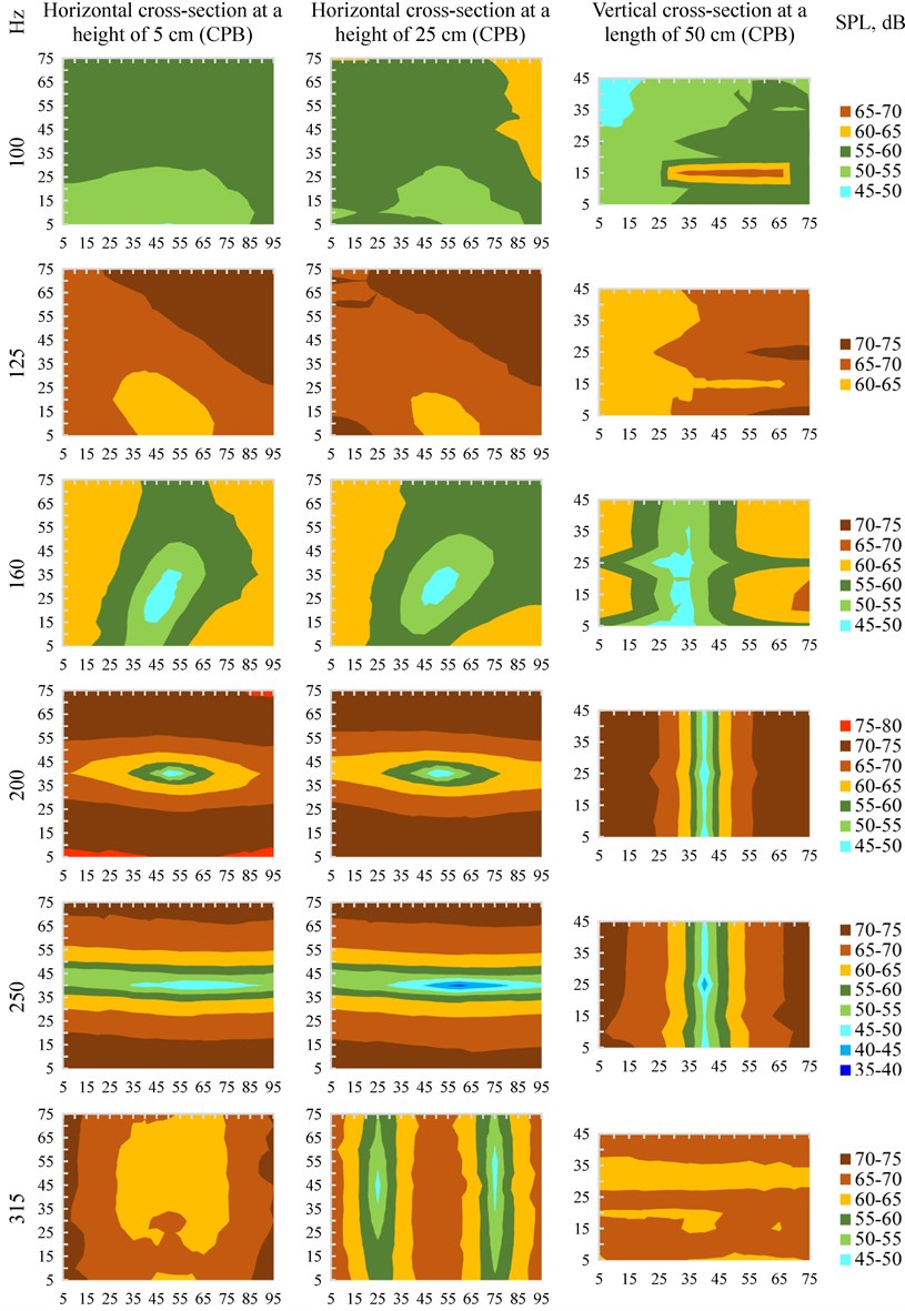
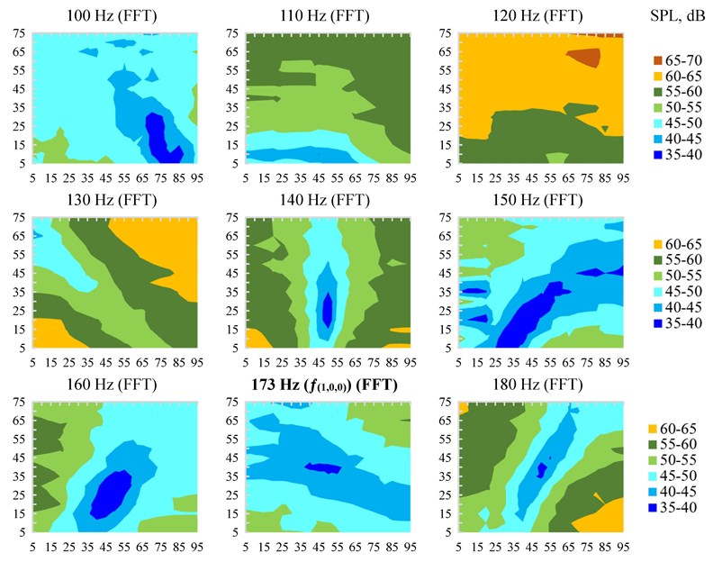
FFT analysis of discrete frequencies in control horizontal cross-sections showed that below the calculated lowest resonant frequency $f_{\left(\mathrm{1,0},0\right)}$, the difference between the highest and lowest sound pressure levels $L_{eq.\left(indr.\right)}$ was even bigger than at $f_{\left(\mathrm{1,0},0\right)}$itself. The spatial distribution of the sound pressure levels at discrete 173 Hz frequency was not clearly expressed and did not repeat the theoretical SPL spatial distribution (an SPL distribution closer to the theoretical one was at 180 Hz or 140 Hz frequencies (see. Fig. 9)). Such differences and spatial distribution of SPLs are attributed to resonant vibrations of the physical model walls.

Fig. 9Variation of measured equivalent sound pressure levels inside the model Leqindr.at a height of 25 cm at discrete frequencies (using the FFT analysis). Note: sound radiation direction is from the bottom of the horizontal cross-sections

At 200-500 Hz centre frequencies in 1/3 octave bands, spatial SPL distribution forms very clear and proportional to the model geometry with large sound pressure level differences were measured (see Fig. 5). Measurements showed that the spatial distribution form of SPLs at 250 Hz centre frequency 1/3 octave band is not similar to the form at a resonant 276 Hz frequency ($f_{\left(\mathrm{1,1},0\right)}$) which is the only resonant frequency at this band (note: according to measurements, the mode becomes clear at higher 278-279 Hz frequencies). This can be explained by the fact that, in performing the sound pressure level measurements, the octave bands cover not only the upper and lower band frequencies, but overlay the closest frequencies at neighbouring bands [15].

At 630-1000 Hz centre frequencies in 1/3 octave bands, due to the large number of modes in one band and the higher line of the modes (as well as smaller differences in the sound pressure levels), a more diffuse acoustic field was obtained. The measurements also showed that the spatial distribution form at 1/3 octave bands was not necessarily similar to the form at discrete centre frequency or resonant frequencies of this band.

Fig. 10Horizontal cross-sections at a height of 25 cm of measured equivalent sound pressure levels Leqindr. distribution inside the model: at 1/3 octave frequencies bands (using CPB analysis), also at discrete centre (of 1/3 octave bands) and resonant frequencies (using FFT analysis). Note: sound radiation direction is from the bottom of the horizontal cross-sections

5. Calculation of sound pressure level inside the model using empirical formulas

Sound pressure levels in a structure are evaluated, in accordance with ISO standard 12354-3 [4], using formulas measuring the volume of the space and the absorbent properties or reverberation time. The calculation can be performed applying a standardised difference of sound levels $D_{2m,nT}$ Eq. (5):

where $L_{\mathrm{1,2}m}$– the average sound pressure level at a distance of 2 m from the façade (in decibels); $T$ – the reverberation time of the space (in seconds); $L_2$ – the average sound pressure level of the space (in decibels); $T_0$ – the reference reverberation time (0.5 s):

where: $V$ – the volume of the space, in our case, equal to 0.4 m³; $S$ – the entire area of the façade, seen from the interior (i.e., the sum of the areas of all the elements of the façade), in our case, equal to 2.6 m²; $\mathrm{\Delta }{L}_{fs}$ – the difference of levels depending on the form of the façade (in decibels), in our case, equal to 0; $R\text{'}$ – sound reduction index or Transmission Loss (TL). It is calculated by summing the strength of the sound directly transmitted by all elements of the façade and the strength of the sound indirectly transmitted. It is held that sound transmission by each element is independent of transmission by the other elements:

where: ${\tau }_{e,i}$ – the ratio of sound transmission between the radiant strength of sound of façade element $i$, caused when impacting this element, and the sound directly radiated in the air, to the strength of sound impacting the entire façade. ${\tau }_f$ – the ratio of sound transmission between the radiant strength of sound of a façade or an indirect element into a space f, caused by transmission of an indirect sound, to the strength of sound impacting the entire façade. In our case, it is insignificant and is not evaluated; $n$ – the number of façade elements directly transmitting sound, $m$ – the number of indirect façade elements and:

where: $R_i$ – the sound reduction index of an individual element (in decibels); $S_i$ – the area of an element $i$ (in square meters).

Because the average sound level in the space is calculated according to the average SPL at the façade, and during the study very different sound levels were measured on the exterior of the model, the calculations were normalised according to the average sound pressure level of the noisiest façade. Normalisation was performed by arithmetically adding the difference between the sound pressure level at the front façade of the model ($L_{eq\left(outdr.40cm\right)frontfacade}$) and the other façade being considered to the separate façade $R_i$. The calculation results are presented in Table 3.

If instead of $L_{eq\left(outdr.40cm\right)}$the values of$L_{eq\left(outdr.avrg.2cm\right)}$ were used, the calculation of $L_{eq\left(indr.avrg.\right)}$would little differ (in an interval from –2.4 dB to 3.4 dB) (see Fig. 11).

Fig. 11Empirically, according to SPL at a distance of 40 cm and 2 cm (Leqoutdr.40cm,Leqoutdr.avrg.2cm) from the front façade (according to ISO 12354-3), calculated (Leqindr.avrg.40cm,Leqindr.avrg.2cm) and, according to measurements, calculated equivalent average SPL Leqindr.avrg.inside the model.

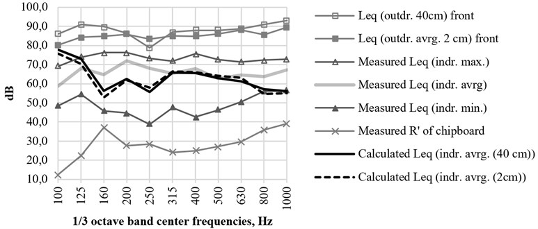
According to the empirical formulas specified in ISO 12354-3, evaluating the average sound level on the exterior of the model, at a distance of 40 cm and 2 cm from the model façades, the calculated sound level inside the model ($L_{eq\left(indr.avrg.\left(40cm\right)\right)}$,$L_{eq\left(indr.avrg.\left(2cm\right)\right)}$) is very similar to that calculated from measurements $L_{eq\left(indr.avrg.\right)}$ in the 315-630 Hz centre frequencies in the 1/3 octave bands (the differences vary from –1.8 dB to 3.4 dB). Measurements in the 160-250 Hz and 800-1000 Hz centre frequencies 1/3 octave bands showed $L_{eq\left(indr.avrg.\right)}$ from 6.6 dB to 12.4 dB higher, and in the 100 Hz band, 16.8-18.8 dB lower. In the 100 Hz band, it was empirically calculated $L_{eq\left(indr.avrg.\left(40cm\right)\right)}\text{,}$$L_{eq\left(indr.avrg.\left(2cm\right)\right)}$larger than measured $L_{eq(indr.max.)}$. Such differences can form due resonances of physical model walls, but can also be affected by inaccuracies of empirical calculations as well as by a non-uniform field in the laboratory hall. In the 800 Hz and 1000 Hz bands, the calculated $L_{eq\left(indr.avrg.\left(40cm\right)\right)}\text{,}$$L_{eq\left(indr.avrg.\left(2cm\right)\right)}$ equals the measured lowest equivalent SPL $L_{eq(indr.min.)}$ and that shows the empirical calculations inadequacy (non-universality)).

6. Calculation of sound pressure level inside the model using FEM

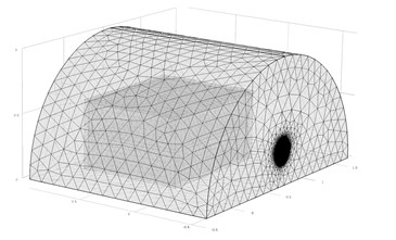
To simulate a situation of investigation above the lowest calculated room mode and to assess differences between average SPLs calculated from measurements and all possible positions, a 3D digital model in COMSOL Multiphysics software (Acoustics model Acoustic-Solid Interaction Frequency Domain) was created. This model solves the Helmholtz equation of plane wave radiation using the finite element method (FEM). The incident plane wave pressure amplitude was defined with respect to measurement results of FFT analysis 2 cm from the front façade. Boundary conditions: plane wave radiation and impedance (for of air), sound hard boundary for floor, fixed constrained (for model bottom). All used to solve equations are included in the software. Tetrahedral mesh size of the FE model was generated with respect to geometry of the model, defining maximum and minimum element size respectively by 10 and 1000 times smaller than the length of the calculated soundwave.

Fig. 12FEM model (and mesh of it) used to simulate investigation

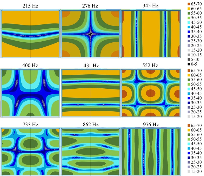
Using FEM calculated equivalent sound pressure levels $L_{eq\left(indr.\right)}$ distribution inside the model is presented in Fig. 13.

Fig. 13Horizontal cross-sections at a height of 25 cm of calculated (using FEM) equivalent sound pressure levels Leqindr. distribution inside the model. Note: sound radiation direction is from the bottom of the horizontal cross-sections

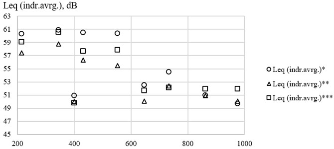
Equivalent average sound pressure levels calculated from measurements at a height of 25 cm of the physical model (FFT analysis) and calculated using FEM equivalent average sound pressure levels at measurement points as well as at whole cross-section and whole model space are presented in Fig. 14.

Fig. 14Equivalent average sound pressure levels: a) * calculated from measurements at a height of 25 cm of the physical model (FFT analysis), b) ** calculated using FEM in the horizontal cross-section at a height of 25 cm, c) ***calculated using FEM at a height of 25 cm from points as in measurements

7. Summary of results

During the study, due to sound source position and sound-reflective surfaces as well as due to dimensions and properties of the laboratory hall, the model was exposed to a non-uniform acoustic field. Non-uniform acoustic field is usually formed in a natural environment. Measurements show, that the difference between equivalent sound pressure levels at a distance of 40 cm (corresponding to a distance of 2 m in a real situation) and 2 cm from model façades ($L_{eq\left(outd.40cm\right)}$-$L_{eq\left(outd.2cm\right)}$) was up to 9.1 dB at the rear (back) façade and up to 6.5 dB at the model’s front façade. These differences are associated exclusively with the microphone position in a non-uniform acoustic field. According to Figure 5, it can be seen that the difference between the calculated equivalent of the sound pressure level at 2 cm from the noisiest (front) façade $L_{eq\left(outd.avrg.2cm\right)}$and the calculated equivalent average sound pressure level $L_{eq\left(indr.avrg.\right)}$in the model ranges from 14.0 to 23.5 dB (the minimum difference was at 200 Hz, and the maximum difference was at 630 Hz centre frequencies 1/3 octave bands). Similarly, the difference between the measured equivalent largest sound pressure levels at 2 cm from the front façade $L_{eq\left(outd.max.2cm\right)}$ and inside the model $L_{eq\left(indr.max.\right)}$ranged from 12.1 to 21.2 dB (the minimum difference was at 160 Hz and the maximum at 630 Hz centre frequencies 1/3 octave bands).

To assess spatial distribution of sound pressure levels $L_{eq.\left(indr.\right)}$ inside the model, measurements were taken every 5 cm starting at 5 cm from the walls across the entire model space (in total, at 2,565 points). Measurements showed that the differences between the highest and lowest equivalent sound pressure levels ($L_{eq.\left(indr.max\right)}$-$L_{eq.\left(indr.max\right)}$) at different 1/3 octave bands were from 16.2 to 34.4 dB. The highest differences were found at 160 Hz, 200 Hz, 250 Hz and 400 Hz centre frequency 1/3 octave bands (see. Fig. 5 and Fig. 6).

The calculated lowest room mode is at 172.5 Hz frequency and falls within the 160 Hz central frequency 1/3 octave band. According to [5], the acoustic field below the calculated lowest resonant frequency should be quite uniform, but it would be true if the walls of the room act as a rigid body. In our case, at lower (100 Hz and 125 Hz centre frequencies) bands, big $L_{eq\left(indr.\right)}$differences (up to 20.7 dB and up to 19.5 dB, respectively) were found and at discrete frequencies (FFT analysis) SPL differences up to 32.4 dB were observed. Such large SPL differences are attributed to resonant vibrations of the physical model walls. From calculations according to equation (4) it can be seen that 5 of the 9 first resonant frequencies ($f_{\left(\mathrm{1,1}\right)}$, $f_{\left(\mathrm{1,2}\right)}$ and $f_{\left(\mathrm{2,1}\right)}$) are between 89.1 Hz (lowest limit of 100 Hz 1/3 octave band) and the lowest room mode ($f_{\left(\mathrm{1,0},0\right)}$) at 172.5 Hz. Spatial SPL distribution at this frequency range has only one region of low sound pressure levels, surrounded by higher levels (see Fig. 9). It should be noted that, as in our case, under natural conditions, a significant difference of SPL below the first resonant frequency is often encountered [16].

In the investigation, even when a sound source outside the physical model forms a non-uniform acoustic field, the measured spatial SPL distribution at all room modes of the physical model (except the lowest room mode $f_{\left(\mathrm{1,0},0\right)}$ (173 Hz)) corresponds to the theoretical spatial variation of sound pressure levels (if the sound source were inside a rigid rectangular space) (see Fig. 10). Inadequacy at $f_{\left(\mathrm{1,0},0\right)}$ (173 Hz) appeared due to possible resonant vibrations of the lateral ($f_{\left(\mathrm{1,2}\right)}$), top and bottom ($f_{\left(\mathrm{2,2}\right)}$) walls of the physical model.

Many countries, in which low frequency noise is regulated, require measuring SPL in a few positions, and one of them should be in the corner (usually 0.5 m from partitions, in our case it corresponds to a distance of 10 cm from the wall), when evaluating low frequency. In the study, calculations were made for equivalent average sound pressure in corners and comparison with average SPL over the model as well as at cross-sections at a height of 20 cm and 30 cm. According to measurements in the corners 5 cm from the wall (and at a height of 45 cm), the calculated average SPL showed that they exceed the average SPL across the model (a total of 2,565 points) up to 6 dB (depending on the frequency band). Average equivalent sound pressure level measured in the corners at 10 cm from the walls (at a height of 40 cm) showed more significant differences from equivalent average SPL in the whole model - the difference depending on the frequency band was from –9.8 dB to 4.2 dB (Fig. 5).

Comparing calculated equivalent sound pressure levels of the entire model with equivalent sound pressure levels in horizontal cross-sections at a height of 20 cm and 30 cm, a difference from 1.1 dB to 3.2 dB at 315-630 Hz centre frequencies bands can be seen, and, respectively, 2.7 dB and 2.6 dB difference at the 100 Hz centre frequency band. At other bands, $L_{eq\left(indr.avrg.\right)}$was similar.From the measurements in corners 5 cm from the walls at a height of 20 cm and 30 cm, the calculated equivalent average SPL differs from calculated average equivalent SPL at the cross-sections from 1.5 to 4.5 dB, and from –1.6 to 5.7 dB, respectively. The calculated average equivalent sound pressure level in the corners 10 cm from the walls differs from average SPLs at the cross-sections from 4.2 to 2.3 and from –4.7 dB to 4.2 dB, respectively (see. Figs. 6 and 7).

FFT analysis at two control cross-sections of the model showed that the equivalent average sound pressure level inside the model $L_{eq\left(indr.\right)}$ at discrete frequencies may vary significantly more than at separate 1/3 octave bands, and the difference between the highest and lowest equivalent average sound pressure levels during the study were up to 49.5 dB (compared to 34.4 dB at 1/3 octave bands).

Performing the study using white noise, that is, using broadband noise, showed that the spatial distribution form (diagram of highest and lowest SPL) of SPLs at the 1/3 octave frequency band differs from spatial SPL distribution (diagram) at discrete centre frequency (FFT analysis). According to the FFT analysis, the acoustic field diagram (spatial distribution of SPL) in room modes was proportional to the model geometry, while at frequencies between the resonant frequencies, spatial SPL distribution has interim forms (transitional spatial SPL distribution from one mode to another), however SPL differences still remain high (above 30 dB).

The sum of discrete SPLs obtained using FFT analysis (from the lower to the upper frequencies of the band) are equal to the sound pressure level at the relevant 1/3 octave band, therefore the more resonant frequencies (modes) are in the relevant band, the more diffuse the acoustic field becomes at the relevant band. The spatial distribution form of SPLs (diagram) at the 1/3 octave band are not necessarily similar to the form at the discrete centre frequency or the form in a given mode.

Indoor SPL variation at low frequencies leads to uncertainties not only in measurements but also in calculations, especially if averaged levels are evaluated. According to the empirical formulas specified in ISO 12354-3 calculations (which evaluates indoor and outdoor average sound pressure levels), conformity between them and equivalent average sound pressure levels calculated according to measurements was found only at 315-630 Hz from all of the 100-1000 Hz range of interest. This means that at frequencies when resonance of walls persists or indoor room modes are forming, calculations using averaged sound pressure levels are not sufficiently accurate.

Calculations with the created model using FEM quite accurately repeated the results for spatial SPL distribution and average sound pressure levels, compared to measurement results using FFT analysis. The average sound pressure levels from FEM calculations and measurements at points along every 5 cm at a height of 25 cm showed differences from –2.3 dB up to 2.8 dB at selected discrete frequencies. Additionally, comparison between the FEM-calculated average sound pressure levels at certain points of measurements and at cross-section at a height of 25 cm showed a difference ranging from –0.2 dB to 2.4 dB. This means that averaging SPL from measurement points along every 5 cm was fairly accurate.

8. Conclusions

Study with a simplified and reduced model permitted simulation of a real situation as to how an acoustic field (SPL differences) can form in a room when the building is exposed to broadband low-frequency sound. Projecting these results to a real potential situation where the object is an empty rectangular room, the following conclusions can be drawn:

1) In the natural environment (as well as in laboratory investigation) large indoor SPL differences below the lowest room mode may be induced by vibration of the building structure or some structural elements at resonant frequencies. At higher bands (than a band with the lowest room mode), spatial SPL distribution mainly depends on model dimensions but also influence of structural resonant vibrations can persist.

2) The study confirms that at outdoor broadband noise, low-frequency sound pressure levels at 1/3 octave bands inside the room can differ by more than 30 dB, while as shown by the FFT analysis, if the noise source emits narrowband sound and sound waves of different frequencies do not interact (do not enter the same band), measured SPL can vary by 50 dB or more (depending on the operating sound level).

3) If the sound waves enter an empty space (room), a spatial distribution of SPL (diagram) in room modes at resonant frequencies forms, proportional to the room geometry, while at frequencies between the resonant frequencies (room modes) the spatial SPL distribution has interim forms (transitional spatial SPL distribution from one mode to another), however SPL differences still remain high.

4) The more resonant frequencies (modes) are in a relevant band, the more diffuse the acoustic field becomes at the 1/3 octave band. The spatial SPL distribution form at the band is not necessarily similar to the form at discrete centre frequency or resonant frequencies of this band.

5) Because in many countries, where low-frequency noise is regulated, it is required to measure SPL at three or more positions and one of them should be in the corner (usually 0.5 m from walls, which in our case is equivalent to a distance of 10 cm from the wall), in the study calculations of equivalent average sound pressure in corners and comparisons with average SPL over the model as well as at cross-sections at a height of 20 cm and 30 cm were carried out. Based on measurements in the corners at a distance of 5 cm from the wall (and at a height of 45 cm), calculated average SPLs showed that they exceed the average SPL across the model (a total of 2,565 points) by up to 6 dB (depending on the frequency band). Average equivalent sound pressure levels measured in the corners at a distance of 10 cm from the walls (at a height of 40 cm) showed even more significant differences from equivalent average SPL in the entire model, the difference depending on the frequency band was from -9.8 dB to 4.2 dB (Fig. 5).

• According to measurements in the corners at a distance of 10 cm from the walls (which correspond to a distance of 0.5 m in a real situation), the calculated equivalent average sound pressure levels vary near curves of average SPL in the entire model or at horizontal cross-sections at a height of 20 cm and 30 cm (the difference of SPLs up to 630-800 Hz bands reaches as high as 2.7 dB). In the corners at a distance of 5 cm from walls (which corresponds to a distance of 0.25 m in a real situation), at almost all bands (except 100 Hz and 125 Hz bands), SPL was measured at levels up to 6 dB higher compared to average levels in the entire model.

In the 1000 Hz centre frequency 1/3 octave band (which corresponds to the 200 Hz band, in which the limit values of regulated sound levels are very low and depending on the country are 10-32 dB [5, 7]) at a height of 40 cm and at a distance of 10 cm from walls in the corner (which corresponds to a distance of 0.5 m from walls and the ceiling), a measured level of equivalent average SPL lower by 9.8 dB than in the equivalent average SPL across the entire model (a total of 2,565 positions). At a height of 30 cm in the cross-section (which corresponds to a height of 1.5 m) in the corners, an SPL lower by an average of 4.6 dB from that of the cross-section was obtained. In the 800 Hz centre frequency band (which corresponds to the 160 Hz frequency band), an SPL lower by 5.9 dB than the average SPL in the entire model was obtained (in this band, the limit values of regulated sound levels are also very low and depending on the country are 14-34 dB [5, 7]).

Calculation of indoor average sound pressure level at frequencies in which indoor room modes form, according to empirical formulas specified in ISO 12354-3 when average SPL near the physical model is used, showed insufficiently accurate results: conformity between measurement and calculation results was found only at 315-630 Hz from across the 100-1000 Hz range of interest.

Calculations using FEM at discrete frequencies can give adequate results of SPL and their spatial distribution. On the other hand, if sound pressure levels at octave (or 1/3 octave) bands are needed, calculation of discrete frequencies and summing of them will be very time-consuming and resource-intensive. FEM calculations produced fairly accurate (from –0.2 dB to 2.4 dB) results, compared with calculated average sound pressure levels at certain points measurement and at cross-section at a height of 25 cm; this means that if indoor low frequencies are investigated, measurements along every 25 cm in a room can produce results close to the average of the sound pressure level of the room.