Abstract
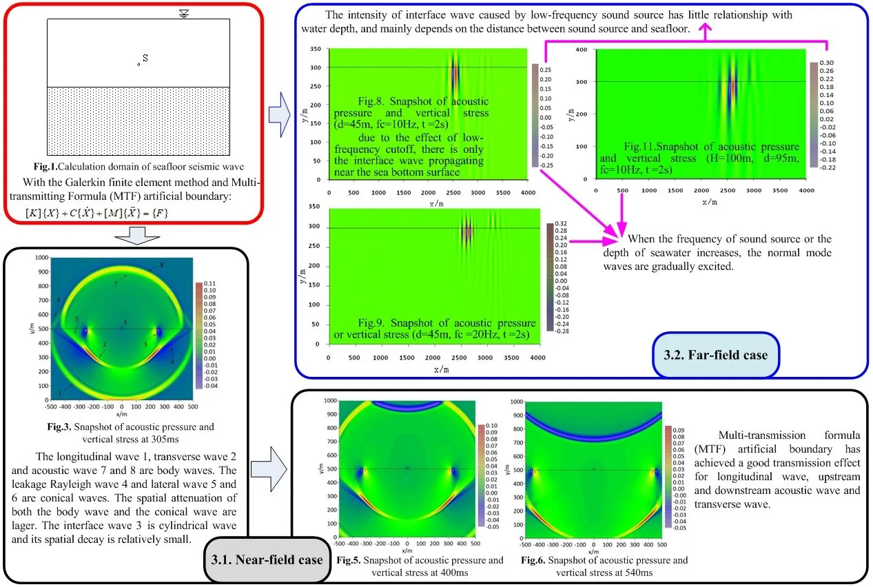
The elastic waves propagating in seabed caused by sailing ships are called ship seismic waves, which can be used to identify ship targets. The wave components and the influences of source frequency, source depth and depth of seawater to the seismic waves are important to the application of seismic wave to detect ship targets. Thus, a forward numerical simulation of seismic waves in shallow sea excited by low frequency sources in time domain was carried out with finite element method based on the Multi-Transmitting Formula artificial boundary. The numerical results show that the body waves and conical waves decay faster in space, but the interface wave decays relatively slow. Multi-transmitting Formula (MTF) artificial boundary has achieved good transmitting effect for longitudinal wave, upstream and downstream acoustic wave and transverse wave. When the source frequency is very low and the seawater layer is shallow, due to the effect of low-frequency cutoff, there is no normal mode wave which can propagate without attenuation in the seawater waveguide, and only the interface wave is propagating near the sea bottom surface. When the frequency of the source or the depth of the seawater layer increases, the effect of low frequency cutoff in the shallow water waveguide is weakened, and the normal mode waves propagating in seawater layer are gradually excited. The intensity of the interface wave caused by low-frequency point sound source mainly depends on the distance between the source and the seafloor.
Highlights
- A forward numerical simulation
- Seismic waves in shallow sea excited by low frequency sources in time domain
- Finite element method based on the Multi-Transmitting Formula artificial boundary
1. Introduction
Seismic wave usually refers to the elastic wave that is caused by the energy released by the crustal activity and propagated to the surface through the stratum. There are mainly three wave forms, namely longitudinal wave, transverse wave and surface wave, whose frequency range is generally below 100 Hz. The hull vibration, the radiation noise of mechanical equipment, the propeller noise and the hydrodynamic noise of sailing ships generates elastic waves propagating along the seafloor outward. The elastic waves propagated to the distant seafloor are called ship seismic waves which can be used to identify ship targets [1-3]. When the frequency of sound source decreases below the cut-off frequency of shallow sea waveguide, there is basically no non-attenuated normal mode wave propagating in shallow sea environment [4], thus it is difficult for traditional sonar to receive ship acoustic signals in the far field. Under this circumstance, the seismic wave caused by the low-frequency noise of ships has become an important way to detect ship targets, which has important application value in the military fields such as the fuse of sea bottom mine and the long-range early warning of quiet submarine [5].
Previous experimental studies investigated the transformation of underwater acoustic radiation into seismo-acoustic waves [6-8]. Theoretically studies of seafloor seismic wave excited by low-frequency acoustic sources also have been done in order to obtain the propagation characteristics of ship seismic waves [9-11]. Among them, the forward numerical simulation in time domain can distinguish the wave components such as longitudinal wave, transverse wave and interface wave, which is favorable to analyze the formation mechanism and propagation process of submarine seismic wave [12-13]. In the above numerical simulation, it is generally necessary to truncate the semi-infinite domain of shallow sea into a finite region and set an absorption boundary at the border of the truncated computational domain. Among this kind of absorption boundary, the Multi-transmitting Formula (MTF) artificial boundary is widely used because of its advantages of small amount of calculation, simple application process and wide adaptability to different waveforms [14-16]. Therefore, based on the Multi-transmitting Formula (MTF) artificial boundary, we carried out forward numerical simulations of shallow sea seismic waves excited by low-frequency sound sources by finite element method in time domain, so as to further clarify the propagation of ship seismic waves. The research will provide a theoretical basis for the application and the development of ship seismic waves in field of underwater target detection.
2. Model of the seismic waves excited by sound sources in shallow sea
For simplification, the noise of ship is regarded as a point sound source, and a simple shallow sea environment consisting of a seawater layer of ideal fluid and a semi-infinite seabed of homogeneous isotropic rock stratum is adopted. For a two-dimensional problem, the wave equations of seismic wave propagating in the seabed are as follows:
where , and are the parameters of the constitutive model of submarine rock stratum; is body force; is density; and are the horizontal and vertical displacements respectively.
The wave equation of acoustic wave in seawater layer is:
where, is sound pressure; is the speed of underwater acoustic wave.
At the acoustic-structure coupling interface, the following fluid-structure interaction relationships are observed:
where, is unit normal vector at the interface is the unit normal vector of interface; is gradient operator; is the gradient operator; is the density of fluid is the fluid density; is the displacement vector is the displacement vector at the interface.
With the Galerkin finite element method, the wave equations of rock stratum and fluid are discretized, and the finite element equation of seafloor seismic wave caused by point sound sources is obtained:
where, is a generalized displacement vector including displacement of rock stratum and sound pressure in fluid, and are velocity and acceleration vectors respectively; , and are stiffness matrix, damping matrix and mass matrix respectively.
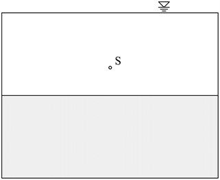
Using the above finite element equation, the numerical simulation of the seafloor seismic waves excited by low frequency point sound source in shallow sea simplified as s two-dimensional ocean environment was carried out in time domain. The calculation domain was shown in Fig. 1. The top boundary is the free surface of seawater. The absorbing boundaries were applied to the left, the right and the bottom boundaries in order to simulate the outer infinite region. The seafloor is the interface of fluid and structure. The point sound source is located at a certain depth in the seawater. The calculation domain was discreted with planar isoparametric element with four nodes. The Newmark implicit integration method was adopted during the numerical integration in time domain. The absorbing boundary is Multi-transmitting Formula (MTF) artificial boundary [17].
Fig. 1Calculation domain of seafloor seismic wave
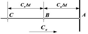
The Multi-transmitting Formula (MTF) belongs to local artificial boundary in time domain. Taking the right boundary in Fig. 1 as example, the multiple transmission formula is:
where represents the displacement or sound pressure of node in Fig. 2 at coordinate and at time ; is order of the multiple transmissions; is an artificial wave speed.
Fig. 2Schematic diagram of multiple transmission formula
In order to analyze the wave components and propagation characteristics of seafloor seismic waves caused by low-frequency sound source, the seismic waves in near-field case and far-field case have been numerically simulated, with a total of 6 numerical examples. The far-field case is defined as the situation where the source and the receiver (or the interest area) are separated by a distance that is more than twenty times the depth of the water. In this case, most of the acoustic rays arriving at the receiver were reflected by the seafloor and sea surface many times, with the water layer acting as a waveguide. The near-field case occurs when the receiver or the interest area are separated from the source by a distance that is almost the same as the depth of sea water. Example 1 and example 2 are near-field cases, which mainly analyze the components of seafloor seismic waves near the sound source. Example 3 - example 6 are far-field cases, which mainly analyze the components of seismic waves far away from the source.
A point sound source emits a wavelet given by:
where is the center frequency, describes the frequency bandwidth of wavelet.
The geo-acoustic properties of two typical sea environments are listed in Table 1.
Table 1Parameters for calculation
Layer | Density (Kg/m3) | P-wave speed (m/s) | S-wave speed (m/s) |
Sea water | 1000 | 1500 | – |
Hard seabed | 2500 | 3000 | 1800 |
Soft seabed | 2000 | 1800 | 1000 |
3. Analysis of the characteristics of seismic waves
3.1. Near-field case
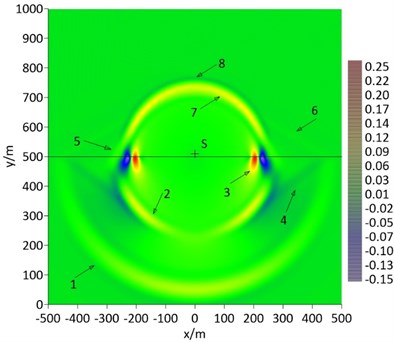
The seabed of numerical example 1 is soft seabed whose S-wave speed is less than the acoustic speed in seawater, the meshed grid size is 2 m×2 m, the time step is 1 ms, the sound source S is located at 10m above the seabed, and the pulse wavelet duration is 0.1 s. Considering the fact that the sound pressure of seawater layer and the vertical stress of seabed are continuous at the seafloor interface, snapshots of the sound pressure-vertical stress in the calculation domain at different times have been shown in figures below. In Fig. 3, the solid black line in the middle represents the seafloor interface, "S" is the sound source, "1" is the longitudinal wave, "2" is the transverse wave, "3" is the interface wave, "4" is the leakage Rayleigh wave, "5" is the lateral wave related to the transverse wave, "6" is the lateral wave related to the longitudinal wave, "7" is the reflected sound wave transmitted upward after the downward sound wave reflected on the seafloor, and "8" is the direct upward sound wave. The longitudinal wave 1, transverse wave 2 and acoustic wave 7 and 8 are body waves. The leakage Rayleigh wave 4 and lateral wave 5 and 6 are conical waves. The spatial attenuation of both the body wave and the conical wave are lager. The interface wave is cylindrical wave and its spatial decay is relatively small.
Fig. 3Snapshot of acoustic pressure and vertical stress at 305 ms
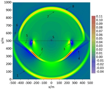
Fig. 4- Fig. 6 show the snapshots of wave field at different time later. It can be seen that the artificial boundary of MTF has achieved a good transmission effect for longitudinal wave (Fig. 4), upstream and downstream acoustic wave (Fig. 5 and Fig. 6), and transverse wave (Fig. 6). Although the transverse wave is slightly reflected in Fig. 6, the slightly reflection is still acceptable in these simulations. Fig. 7 shows the snapshot of wave field in example 2 with a hard seabed whose S-wave speed is greater than the acoustic speed in seawater. The wave composition is similar to that of the soft seabed, except that the velocity of transverse wave is greater than the acoustic speed in seawater.
Fig. 4Snapshot of acoustic pressure and vertical stress at 350 ms
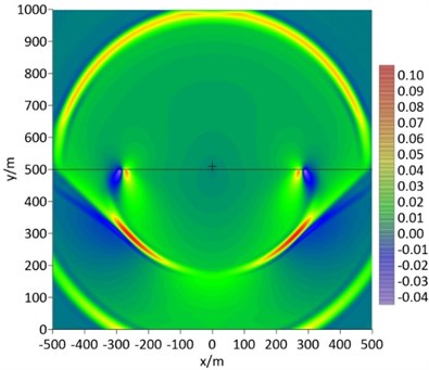
Fig. 5Snapshot of acoustic pressure and vertical stress at 400 ms
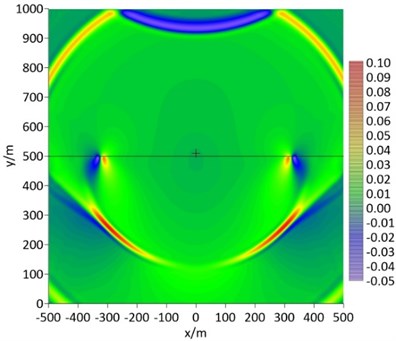
Fig. 6Snapshot of acoustic pressure and vertical stress at 540 ms
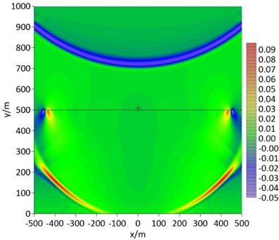
Fig. 7Snapshot of acoustic pressure and vertical stress at 180 ms (hard seabed)
3.2. Far-field case
In order to analyze the wave components and propagation characteristics of seismic waves in far-field excited by low-frequency acoustic sources, four numerical simulations have been carried out in a typical shallow sea with hard seabed. The width of the calculation domain is 4000 m, and the depth of seawater layer in example 3 and example 4 is 50 m, while the depth in example 5 and example 6 was increased to 100 m in order to analyze the influence of seawater depth to the propagation characteristics of seismic wave.
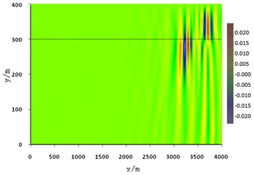
In example 3, the center frequency of the pulse wavelet of the sound source is 10 Hz, the bandwidth is 20 Hz, and the depth of the sound source is 45 m. Fig. 8 is the snapshot of example 3 at 2 s. In this figure, we can see that only a wave group propagating along the seafloor in the range of about 2500 m. The wave group has the largest sound pressure or vertical stress near the seafloor surface, and decays rapidly with the distance away from the seafloor surface. The above distribution characteristics conform to the spatial distribution characteristics of interface wave. Thus, the wave group propagating along the seafloor in Fig. 8 is considered as interface wave propagating along the seafloor. It can be seen that when the frequency of the sound source is very low and the depth of seawater is shallow, due to the effect of low-frequency cutoff, there is no normal mode wave propagating without attenuation in the waveguide of seawater, and only the interface wave propagating near the sea bottom surface.
Fig. 8Snapshot of acoustic pressure and vertical stress (d= 45 m, fc= 10 Hz, t= 2 s)
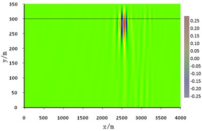
Fig. 9Snapshot of acoustic pressure or vertical stress (d= 45 m, fc= 20 Hz, t= 2 s)
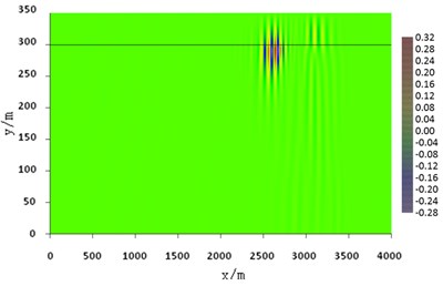
When the center frequency of sound source increased to 20 Hz in example 4, the snapshot of sound pressure-vertical stress was shown in Fig. 9. A new wave group appears in front of the interface wave, and its spatial distribution of amplitude is obviously different from that of the interface wave. The maximum value of the sound pressure lies in the middle of the seawater waveguide, which conforms to the propagation characteristics of the first-order normal mode wave. Thus, when the frequency of the sound source increases, the effect of low-frequency cutoff in the shallow sea waveguide weakens and the normal mode waves are gradually excited.
The frequency dispersion curve is an efficient tool to analyze the phase speed and group speed of guide wave [18]. According to the normal-mode theory, the dispersion relation for the normal modes can be derived by setting the determinant of global coefficient matrix of the depth-separated wave equations in frequency-wave numbers domain to zero [19]:
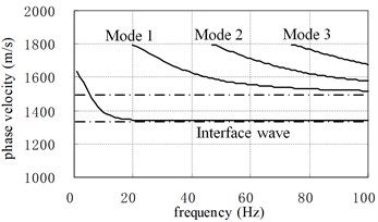
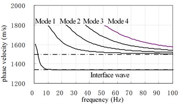
The real roots of Eq. (8) correspond to normal modes propagating without leaking energy away from the waveguide. These normal models can be further classified into interface wave propagating along the seafloor and normal modes propagating in the waveguide of shallow sea. After finding all the real roots of dispersion relation Eq. (8), we plotted the dispersion curves of the above example 3- example 4 as Fig. 10.
As shown in Fig. 10, there are interface wave and several normal modes displayed in the dispersion curves. Each normal mode has a well-defined low-frequency cutoff while the interface wave almost does not. Thus, the time series of the seismic wave in example 3 is dominated by the interface wave when the source frequency is less than the minimal cut-off frequency of the first-order normal mode wave (0-20 Hz, 10 Hz, bandwidth of wavelet is 20 Hz). In example 4, the first-order normal mode wave appears when the source frequency increases and passes its cut-off frequencies (10-30 Hz, 20 Hz, bandwidth of wavelet is also 20 Hz).
In example 5, the depth of seawater layer was increased to 100 m, and the other calculation parameters were kept the same as example 3, so as to analyze the influence of seawater depth. The snapshot of sound pressure-vertical stress was shown in Fig. 11.
Fig. 10Dispersion characteristics of phase velocity (H= 50 m, hard seabed)
Similar to Fig. 9, a new wave group appears in front of the seafloor interface wave in Fig. 11, which is mainly propagating in the waveguide of the seawater and should be the first-order normal mode wave. Thus, when the depth of seawater increases, the effect of low-frequency cutoff in the shallow sea waveguide will also weaken, and normal mode wave is gradually excited.
Of course, due to the very close distance between the sound source and the seafloor, the amplitude of the interface wave is relatively strong, and the normal mode wave is relatively weak and not clear in Fig. 11. In Fig. 11, the intensity of interface wave is almost the same as that of example 3 with 50 m water depth, which indicates that the intensity of interface wave caused by low-frequency sound source has little relationship with water depth, and mainly depends on the distance between sound source and seafloor.
In example 6, the sound source was moved far away from the seafloor surface and located at 10 m below the water surface. The snapshot of sound pressure-vertical stress was shown in Fig. 12. The amplitude of the interface wave decreases significantly by nearly one order of magnitude compared with Fig. 11, while the amplitude of the normal mode wave does not change much. Therefore, both the normal mode wave and the interface wave are clearly displayed in the snapshot.
Fig. 11Snapshot of acoustic pressure and vertical stress (H= 100 m, d= 95 m, fc= 10 Hz, t= 2 s)
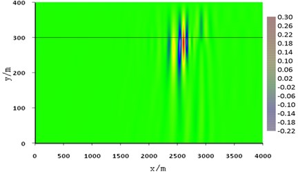
Fig. 12Snapshot of acoustic pressure or vertical stress (H= 100 m, d= 10 m, fc= 10 Hz, t= 2.5 s)
Similarly, we plotted the dispersion curves of the above example 5- example 6 as Fig. 13.
Compared with Fig. 10, it is clear that the cutoff frequency of each normal mode decreases and more normal modes appear when the depth of sea water increases to 100 m. Thus, in example 5 and example 6, the first-order normal mode wave appears although the source frequency is very low (0-20 Hz, 10 Hz, bandwidth of wavelet is also 20 Hz).
Fig. 13Dispersion characteristics of phase velocity (H= 100 m, hard seabed)
4. Conclusions
Based on the established calculation model, the seafloor seismic waves excited by low frequency point sound sources in two-dimensional liquid-solid semi-infinite space were simulated. The wave components and the propagating properties of ship seismic wave in shallow sea were analyzed according to the simulating results. The influences of source frequency, source depth and depth of seawater to the seismic waves have been discussed in this paper. The results show that:
1) The longitudinal wave, transverse wave and acoustic wave are body waves, while the leakage Rayleigh wave and lateral waves are conical waves. The spatial attenuation of both the body wave and the conical wave are lager. The interface wave is cylindrical wave and its spatial decay is relatively small.
2) Multi-transmission formula (MTF) artificial boundary has achieved a good transmission effect for longitudinal wave, upstream and downstream acoustic wave and transverse wave. Although the transverse wave is slightly reflected, the slightly reflection is still acceptable in the simulations.
3) In a typical shallow sea with hard seabed, when the frequency of the sound source is very low and the depth of seawater is shallow, due to the effect of low-frequency cutoff, there is no normal mode wave propagating without attenuation in the waveguide of seawater, and only the interface wave propagating near the sea bottom surface.
4) When the frequency of sound source or the depth of seawater increases, the effect of low-frequency cutoff in the shallow sea waveguide weakens and the normal mode waves are gradually excited.
5) The intensity of interface wave caused by low-frequency sound source has little relationship with water depth, and mainly depends on the distance between sound source and seafloor.
In this paper, the wave components and the propagation properties of ship seismic waves in shallow water were discussed by numerical simulation combined with dispersion curves of the depth-separated wave equations. Due to financial constraints and difficulties in sea trial, we did not conduct sea trial to validate the numerical results with experimental data. This would be one of our future works. Furthermore, the real shallow sea environment is relatively complex, which is mostly composed of several strata of rock and soil, and each layer generally is absorbing attenuated. Therefore, the above theoretical analysis of seafloor seismic waves caused by radiation noise of ship needs to be further studied in consideration of multi-layers medium in seabed and the absorption attenuation in strata of rock and soil.
References
-
A. I. Mashoshin, “Optimization of a device for detecting and measuring parameters of amplitude modulation of underwater noise emission of seagoing vessels,” Acoustical Physics, Vol. 59, No. 3, pp. 305–311, May 2013, https://doi.org/10.1134/s106377101303010x
-
Z.-H. Lu, Z.-H. Zhang, and J.-N. Gu, “Analysis on the synthetic seismograms of seismic wave caused by low frequency sound source in shallow sea with porous seabed,” Journal of Theoretical and Computational Acoustics, Vol. 26, No. 4, p. 1850001, Dec. 2018, https://doi.org/10.1142/s2591728518500019
-
A. E. Borodin, A. G. Dolgikh, G. I. Dolgikh, and V. K. Fishchenko, “Recording seismoacoustic signals of a surface vessel with a two-coordinate strainmeter,” Acoustical Physics, Vol. 62, No. 1, pp. 64–73, Jan. 2016, https://doi.org/10.1134/s1063771015060020
-
F. B. Jensen, W. A. Kuperman, M. B. Porter, and H. Schmidt, Computational Ocean Acoustics. New York, NY: Springer New York, 2011, https://doi.org/10.1007/978-1-4419-8678-8
-
Meng Lu-Wen, Cheng Guang-Li, Chen Ya-Nan, and Zhang Ming-Min, “On the Porpogation Mechanism of Ship Seismic Wave and Its Application in Mine Fuze,” Acta Armamentarii, Vol. 38, No. 2, p. 319, Apr. 2017, https://doi.org/10.3969/j.issn.1000-1093.2017.02.016
-
V. S. Averbakh et al., “Application of hydroacoustic radiators for the generation of seismic waves,” Acoustical Physics, Vol. 48, No. 2, pp. 121–127, Mar. 2002, https://doi.org/10.1134/1.1460944
-
G. I. Dolgikh, “Experimental estimate for the transformation of underwater acoustic radiation into a seismoacoustic wave,” Acoustical Physics, Vol. 51, No. 5, pp. 538–542, 2005, https://doi.org/10.1134/1.2042572
-
R. Stephen et al., “The ocean bottom seismometer augmentation of the Philippine Sea experiment,” The Journal of the Acoustical Society of America, Vol. 131, No. 4, pp. 3352–3352, Apr. 2012, https://doi.org/10.1121/1.4708564
-
X. Li and B. Yan, “Ships seismic-wave field influenced by the characteristic of different marine sediment,” Ship Science and Technology, Vol. 30, No. 4, pp. 43–46, 2008.
-
Z.-H. Lu, Z.-H. Zhang, and J.-N. Gu, “Numerical calculation of seafloor synthetic seismograms caused by low frequency point sound source,” Defence Technology, Vol. 9, No. 2, pp. 98–104, Jun. 2013, https://doi.org/10.1016/j.dt.2012.12.001
-
Yang Shi-E., “Propagation of seismic waves caused by underwater infrasound,” Journal of Harbin Engineer University, Vol. 31, No. 7, pp. 879–887, 2010.
-
Z. Lu, Z. Zhang, and J. Gu, “Modeling of low-frequency seismic waves in a shallow sea using the staggered grid difference method,” Chinese Journal of Oceanology and Limnology, Vol. 35, No. 5, pp. 1010–1017, Sep. 2017, https://doi.org/10.1007/s00343-017-6026-4
-
L. W. Meng, X. Y. Luo, and G. L. Cheng, “Components and propagation characteristics of seabed seismic waves,” Journal of Shanghai Jiao Tong University, Vol. 52, No. 12, pp. 1627–1633, 2018.
-
H. Xing, X. Li, H. Li, and A. Liu, “Spectral-element formulation of multi-transmitting formula and its accuracy and stability in 1D and 2D seismic wave modeling,” Soil Dynamics and Earthquake Engineering, Vol. 140, p. 106218, Jan. 2021, https://doi.org/10.1016/j.soildyn.2020.106218
-
V. Kumar*, S. Rani, A. Priyadarshee, A. Kumar, and A. K. Rahul, “Effect of transmitting boundary on soil – slope – foundation interaction,” International Journal of Innovative Technology and Exploring Engineering, Vol. 9, No. 4, pp. 3130–3136, Feb. 2020, https://doi.org/10.35940/ijitee.d1406.029420
-
J. Su, Z. Zhou, Y. Li, B. Hao, Q. Dong, and X. Li, “A stable implementation measure of multi-transmitting formula in the numerical simulation of wave motion,” PLOS ONE, Vol. 15, No. 12, p. e0243979, Dec. 2020, https://doi.org/10.1371/journal.pone.0243979
-
Z. P. Liao and Z. N. Xie, “Stability of numerical simulation of wave motion,” Journal of Harbin Engineering University, Vol. 32, No. 9, 2011.
-
M. Roth, K. Holliger, and A. G. Green, “Guided waves in near-surface seismic surveys,” Geophysical Research Letters, Vol. 25, No. 7, pp. 1071–1074, Apr. 1998, https://doi.org/10.1029/98gl00549
-
J. O. Parra and P. C. Xu, “Dispersion and attenuation of acoustic guided waves in layered fluid‐filled porous media,” The Journal of the Acoustical Society of America, Vol. 95, No. 1, pp. 91–98, Jan. 1994, https://doi.org/10.1121/1.408269
About this article

This work was supported in part by the National Natural Science Foundation of China, Grant No. 51179195 and 51679248.
The datasets generated during and/or analyzed during the current study are available from the corresponding author on reasonable request.
The authors declare that they have no conflict of interest.
