The modal analysis of disc resonator gyroscope using isogeometric analysis

1. Introduction

With the widespread application of microelectromechanical system (MEMS) gyros especially in automotive safety and military tactical, researchers keep trying to find the high performance MEMES gyros [1-5]. The Hemispherical Resonator Gyroscope (HRG) is known as one of the highest performance gyroscopes thanks to inherent advantages of a degenerate wineglass mode operation such as thermal stability, electrostatic tuning capability, and high quality factor [6, 7]. However, the early resonator designs set stringent requirements on complex control strategy such as close-loop force feedback and mode-tuning, ultra-low noise electronics design, high cost 3D assembly technique in improving the capacitive sensitivity. In addition, the gyro bias was not stable due to the high dynamic load and imprecision of the bonded joints when running long. Given this background, the conception of the Disc Resonator Gyroscope (DRG) was proposed which yielded a compact planar micro-machined design with central support and carrying no critical loads [8-10].

The optimization of structural parameters and material selection has made contributions to achieve much stable performance, and this work is still in progress. The current approach of modal analysis is usually based on the FEM software including three steps: building the geometric model, transforming the geometry into mesh and making the modal analysis. It means that in every optimization cycle, the model will be modified once and re-meshed to analyze which brings a lot of repetitive work.

The concept of Isogeometric Analysis was firstly proposed by Hughes et al. [11] in 2005. It seeks to unify the fields of the computer-aided design (CAD) and the finite element analysis (FEA). The root idea is that the basis used to exactly model the geometry will also serve as the basis for the solution space of the numerical method. On this base, the model used for analysis is automatically created from CAD geometry and the procedure from geometry to mesh is skipped which reduces the repetitive work. On the other hand, the mesh refinement in IGA does not change the geometry which ensures the unification of geometry and analysis [12-14]. The application of IGA to structural vibration was firstly introduced by Cottrell et al. [15]. Since then, a various number of researches employing IGA approach have been presented to solve the dynamic problem in a wide range of research areas.

In this context, the advantages of IGA approach are employed to determine the intrinsic frequencies and the mode shapes for the DRG. When designing a DRG, the overall structure will not change except the size and material parameters. It provides convenience for the optimization because the procedure can be parameterized by using IGA. Moreover, the NURBS can exactly describe the circular geometry even at coarse mesh level. The main body of the DRG is composed of rings which means the IGA will offer an effective and accurate calculation.

In this work, we don’t focus on how to design a DRG with good performance but the modal simulation of DRG using IGA which is the basis of optimization. This paper is organized as follows:

Section 2 gives a brief introduction to the NURBS discretization and the free vibration analysis. Section 3 presents the structure of DRG and the analysis model. Section 4 shows the simulation results and comparison and Section 5 concludes this paper.

2. NURBS-based discretization and Free vibration analysis

Here we briefly review the concept of NURBS. For further details and extensive references, the reader is referred to Piegl and Tiller and Cottrell et al. [16-20].

A NURBS curve $\mathbf{C}\left(u\right)$ can be described as:

where $R_{i,p}\left(u\right)$ are the NURBS basis functions, ${\mathbf{P}}_i$ are the control points, $w_i$ are the weights of the control points, $\mathbf{U}={\left\{u_1=0,\cdots ,u_i,\cdots ,u_{n+p+1}=1\right\}}^T$is the knot vector in the parameter space, $p$ is the polynomial order [21].

Taking the form of Eq. (1), the related reference coordinate and displacement located in the control point can be defined as:

where $n_{cp}$ is the number of control points, $R_A$ is the NURBS basis function corresponding to control point $A$.

For 2D problem, the Green strain is expressed as:

where $\mathbf{B}$ is the strain-displacement matrix, $\mathbf{J}$ is the Jacobian mapping physical and parametric domains. $(x_i,y_i)$ are the coordinates of control points.

Thus, for a body defined in the domain $\mathrm{\Omega }$, we can get the stiffness matrix and the mass matrix as:

where $\mathbf{D}$ is the elastic matrix, $\rho$ is the material density and $t$ is the thickness.

To compute the natural frequency, we ignore the damping matrix and the load vector. Thus, the global equation of motion for the DRG system can be written as:

where $\mathbf{M}$ is the global mass matrix, $\mathbf{K}$ is the global stiffness matrix and $\mathbf{U}=\{u_1^1,u_1^2,\cdots ,u_n^1,u_n^2\}$ is the global displacement vector (the superscript of $u_i^{\mathrm{1,2}}$ is the direction of DOF and n is the number of control points).

By assuming $\mathbf{U}=e^{i\omega t}\stackrel{-}{\mathbf{U}}$, the motion equation is:

Then, it can be translated into the eigenvalue problem:

where $\stackrel{-}{\mathbf{U}}$ is the associated displacement vector and the solution of Eq. (12) is the natural frequency.

3. DRG model

The DRG is constructed by a series of rings and connected with spokes. Fig. 1(a) gives the picture of real product and Fig. 1(b) shows a design schematic diagram of DRG [7]. In the actual model, there is a fixed solid disk in the center as shown in Fig. 1(b). For the analysis model, we fixed the most inside spokes instead and set it as the displacement boundary condition as shown in Fig. 2(a). The details of the control points and the mesh are shown in Fig. 2(b) and Fig. 2(c).

Fig. 1The structure of DRG: a) shows a real model, for b), the solid blue lines represent spokes that are fixed, while the dashed red lines represent spokes that are variable

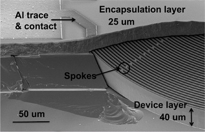
a) SEM image of epi-sealed DRG

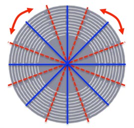
b) The design sketch

To obtain the analysis model in the traditional FEA, we should draw the model first and transform it into mesh then. If we want to change the number of the rings or other parameters, these two steps have to be repeated. Here we give a detailed introduction of the modeling process using IGA which is parameterized.

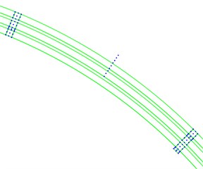
The tensor product structure of the parameter space of a patch makes it poorly suited for representing complex, multiply connected domains [12]. The DRG can be handled by using multiple patches as shown in Fig. 2(c).

Fig. 2The sketchy analysis model: a) is the diagram, b) shows the control points (blue points), c) shows the multiple patches and the green lines constitute the mesh

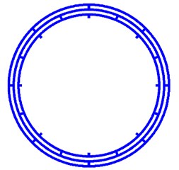
a)

b)

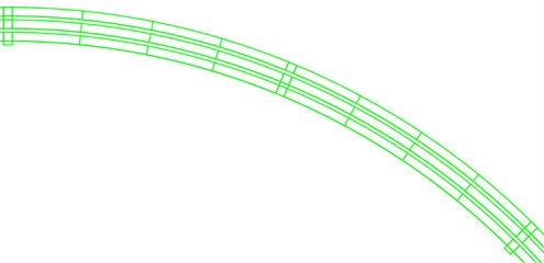
c)

If we set every spoke as a patch, there are 8 patches inside every ring which can be divided into 32 patches. Table 1 lists the number of patches associated with the number of rings. Table 2 gives the parameters set in the simulation model of DRG.

The internal diameter of each ring can be derived based on the ring width and the electrode gap size, then, the control points’ coordinates of all the patches can also be calculated. Due to the model is completely based on the parameters given in Table 1 and Table 2, we only need to change the parameters at the beginning of the model process and the model modification will be automatically generated.

Fig. 3 shows the analysis models with different number of rings (10 rings and 35 rings) and the only thing to change is the parameter $N_r$ in the whole modeling process. For the convenience of calculation and the modeling in ABAQUS, we choose the model of 3 rings in the numerical simulation as an example.

Fig. 3a) is the model of 10 rings, b) is the model of 35 rings

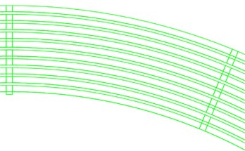
a)

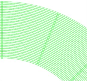
b)

4. Numerical results and comparison

In order to verifies the IGA model, ABAQUS is selected to compare the simulation results between IGA and FEM. In the comparison, four different meshes are employed in each method, the first ten natural frequencies and mode shapes are computed and we assume that the result of highly refined model (387104 nodes) in ABAQUS is the standard value. The results are separately shown in Table 3 and Table 4 (The unit of all the frequencies is Hz).

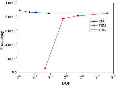
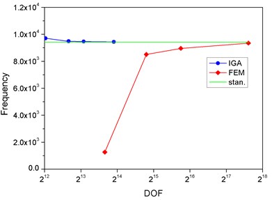
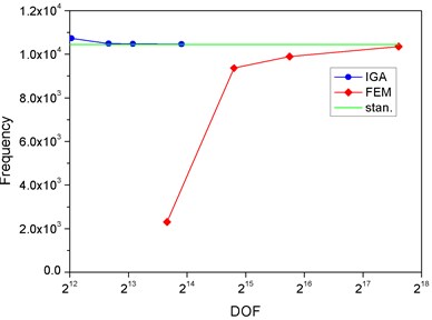
For further comparison, we choose the value of the frequency of fundamental, 2nd order, 4th order and 10th order harmonics, respectively. The correlation curves are shown in Fig. 4(a), (b), (c) and (d). Because of the large span of the abscissa, we take the format of log 2. The first ten mode shapes are shown in Fig. 5. The relative error of the second frequency between IGA and FEM is given in Table 5.

Fig. 4The correlation curves in four different modes

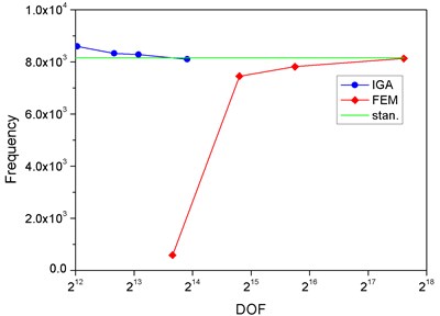
a) Mode 1

b) Mode 2

c) Mode 5

d) Mode 10

Obviously, we find that, the DOF in IGA is much less than FEM to approach the standard value. In the finite element method, the DOF will directly affect the solution time. Therefore, it proves that the computational efficiency of IGA is higher than FEM. Table 5 also shows the high accuracy of IGA when the DOF is relatively less.

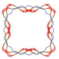
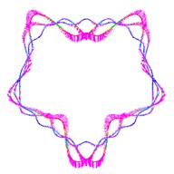
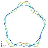
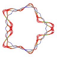
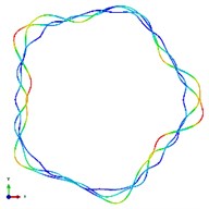
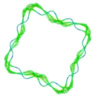
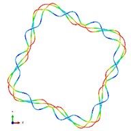
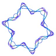
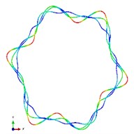
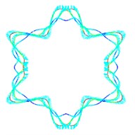
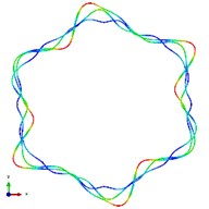
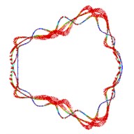
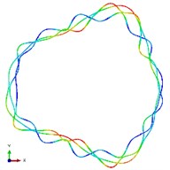
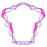
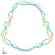
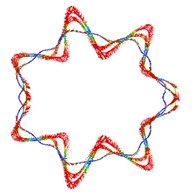
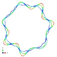
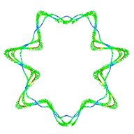
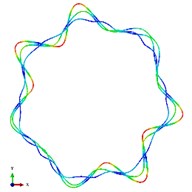
Fig. 5The first ten mode shapes. a)-j) show the mode shapes from 1st to 10th, the left one of each part is the result of IGA (drawn by Tecplot), the right one is the result of ABAQUS

a1)

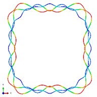
a2)

b1)

b2)

c1)

c2)

d1)

d2)

e1)

e2)

f1)

f2)

g1)

g2)

h1)

h2)

i1)

i2)

j1)

j2)

5. Conclusions

In this work, the Isogeometric analysis based on NURBS is applied in the modal simulation for the disc resonator gyroscope (DRG). It provides two advantages:

• NURBS geometry is more efficient in describing circular structure and it provides higher accuracy and efficiency.

• It’s uniform between design and analysis which means there is no need to re-mesh the model in the optimization period. It can save a lot of repeated work in the optimization design.

Four different level of mesh refinements are computed by using IGA and ABAQUS in the numerical example. The results of first ten frequencies and mode shapes are analyzed to compare the efficiency and accuracy. The method of Isogeometric analysis shows great advantages.

The extension to three-dimension analysis is the ongoing research [22]. Also, we are trying to design a better performance DRG by using IGA and compare with physical experiment.