Abstract
For objects of “large” vibration size such as waves on the sea surface, the choice of measurement method can create different understandings of system behavior. In one case, laser vibrometry measurements of a vibrating bar in a controlled laboratory setting, variation in probe spot size can omit or uncover crucial structural vibration mode coupling data. In another case, a finite element simulation of laser vibrometry measures a nonlinearly clattering armor plate system of a ground vehicle. The simulation shows that sensing the system dynamics simultaneously over the entire structure reveals more vibration data than point measurements using a small diameter laser beam spot, regardless of the variation of footprint (coverage) boundaries. Furthermore, a simulation method described herein allows calculation of transition probabilities between modes (change-of-state). Wideband results of both cases demonstrate the 1/ trend explained within – that the energy of discrete structural vibration modes tends to decrease with increasing mode number (and frequency), and why. These results quantify the use of less expensive non-imaging classification systems for vehicle identification using the remote sensing of surface vibrations while mitigating spectral response distortion due to coverage variation on the order of the structural wavelength (spectral reduction or elimination).
Highlights
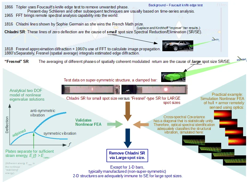
- Test data shows the small spot size return of vibrating plates is susceptible to spectral elimination (SE) on the Chladni lines, shown by Sophie Germain in 1816 to have no normal motion.
- Test data shows the large spot size return from vibrating plates is susceptible to spectral reduction (SR) due to spatial averaging over the illuminated coverage area.
- Except for 1-D vibrations (bar, rod, or thin slat), super-symmetric structures have an optical return susceptible SE, the severe subset of SR.
- An example of vibrating plates with nonlinear contact provided FEA output for MATLAB image propagation resulting in a cross-spectral covariance of structural to optical spectra.
- An extensive nonlinear mechanics analytical calculation provides the nonlinear eigen-states for clattering plates as two masses in contact sufficient to validate modal results of the structural FEA.
- Since super-symmetric 2-D and 3-D structures are impractical to manufacture, typical manufactured structures may suffer modest SR but are effectively immune to SE.
1. Introduction
Remote vibrometry has many forms. The use of optics to sense vibration is a mature technology that dates back to methods of observations with knife-edge imaging invented by Jean Bernard Léon Foucault in 1858 that can be used to measure mirror shape. The method was also used by Töpler [1] in 1866 to measure phase and later used to remove unwanted optical phase effects: “the Schlieren method, where all the spectra on one side of the central order are excluded”. [2] The Schlieren method, a German word for streak, uses Foucault’s knife-edge in the “Fourier plane” at a distance of a focal length from a collecting lens. A related method, the streak tube, can optically process an entire slice of underwater scenery nearly instantaneously [3-5]. More recent physics discoveries use vibration to measure atomic size effects. Microscopy resolution smaller than the optical diffraction limit can be accomplished with the Nobel prize winning [6] scanning tunneling microscope. Other microscopes image S-shells of large atoms and, in some atoms, their P-shells. The microscopic range, remote vibrometry variant, the atomic force microscope (AFM) is able to detect separate molecules by measuring the difference in van der Waals force as a tiny vibrating cantilever sensitive to the atomic outer shell locations, scans over the sample. These are some examples of remote vibrometry. This article describes how the nature of observations can provide different pictures of the vibrational modes of common vehicles and other integrated structures built from plates, shells, and membranes (the “body-in-white”).
Three types of analysis provide support for this investigation of observation methods for structural surface waves. (i) Experimental results of a driven clamped bar with full fixity at both ends provides a laser vibrometry spectrum for both small and large probe beam spot sizes. (ii) The author’s master’s thesis [7] contains calculation results of imaging a vehicle hull at 4 kilometers. Identification of the target vehicles is based on spectral fingerprints formed from laser vibrometry. The target armor clattering against the vehicle hull provides a surface vibration that modulates the probe beam. (iii) Several analytical calculations using explicitly nonlinear mechanics validate the distinct clattering spectrum. These experimental, simulation, and analytical results provide cross-supporting reinforcement for the three observational characteristics described in this work.
This work defines three characteristics of composite structures such as vehicles. (1) The lower frequency modes are nearly discrete. (2) Energy from driven modes flows into other modes. And finally, (3) due to theory and observations defined herein, vibration strain-energy is higher in the fundamental mode, with energy decreasing as modal frequencies increase. The latter two characteristics can be considered [8] to be consequences [9] of the second law of thermodynamics.
The probe beam spot size affects vibration modes that are observed with optics. Some vibration modes may not be obvious from return due to a probe beam with a small spot size, as discussed with Flight Lieutenant Ngoya Pepela’s thesis [10] in Figs. 5 and 6 for a vibrating bar. In the simulation of clattering armor plates, more mode information is acquired when viewing the entire optical image and processing its spectrum at multiple locations. In spite of some interference, the non-imaging (spatially integrated radiant flux) spectrum of the probe return from the entire target’s surface provides more information than the small spot size in that phase information over time is embedded in the sensed signal [7].
1.1. Three observational characteristics
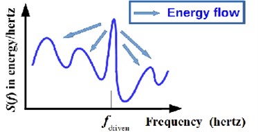
Based on the three previously mentioned supporting results, the experiments, simulation, and analytical results, three observations become apparent: (1) the lower frequency modes have sharp resonances that are effectively discrete responses. Fig. 1 is a sketch of a notional representation of this case. These modes can be modeled on center frequencies when damping is limited to structural damping [11], as later discussed in Fig. 5 and 6. (2) Energy transfers from one structural component and its vibration modes into the lower modes of nearby components through joints, including welds, which have nonlinear load-deflection curves. Each mode is comprised of a 3-D mode shape (deflection vectors) of the entire structure (Fig. 2). The strain-energy (modal energy) of each mode couples to lower energy modes as the system transforms from transient to steady state. Finally, (3) modal energy flows into the lowest frequencies first, saturating them (Fig. 3), depleting the energy flow as the mode number increases from , , ,… and up through the closely-spaced high frequency modes that become practically infinite in density. For discrete modes the finite element analysis (FEA) results are limited to the number of degrees of freedom (DOF) in the model.
The energy at each of the modes shown in the notional sketch (Fig. 1) transfers to lower energy modes if physical load paths exist that are conducive to mode coupling. These sketches summarize decades of trade secret testing. At least one example appears in the literature for automotive modal analysis, ride and handling [12]. Helicopter data is available from MIL-HDBK-810 [13]. A transfer of energy from a strongly driven mode to other modes appears in Fig. 2. That driver might be in a component located far from the receiving modes [14], but in “frequency space” these modes might be coupled. Vibrations might be driven by the engine at one frequency, yet sensed in the back seat at another frequency. Nonlinearities in response can create harmonics of resonances that allow energy to couple with lower modes. The low energy tails of wide resonances (damped broadening) also “touch” other modes of lower frequencies. Another energy transfer mechanism occurs in clattering plates where spatial distribution of mode amplitudes causes contact that excites different modes. This transfer of energy is much similar to plucking a musical string at different locations to change the overall sound. Energy transfer between states depends on the frequency of the mode, which is the square root of the eigenvalue in an analysis of normal modes.
Fig. 1The lowest frequency modes have high resonance quality Q compared to high frequency response, unless systems have large damping on these “lower” modes or frequency-dependent control systems. For adequate signal to noise ratios, these frequencies identify what are effectively discrete modes, as represented in the stem chart to the right
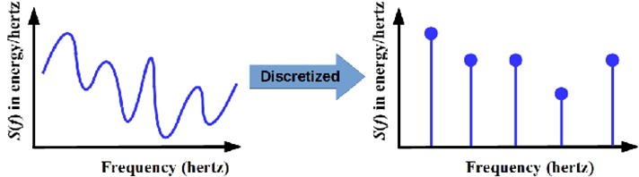
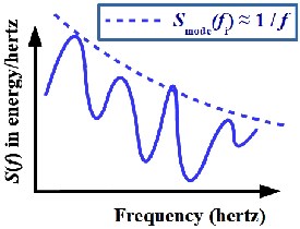
Fig. 3 is a sketch where the final steady state of the vibrational system has energy ordered from strong resonances at the fundamental frequency to a paucity of energy at higher frequencies. A quote from Zienkiewicz, displayed later in Section 3, provides an explanation for this common 1/ dependence of modal energy. The exceptions noted also include strong damping or added mass.
Fig. 2Vibrational strain-energy from different components transfers from a driven mode, the indicated most powerful response, to lower energy modes at different frequencies. For example, the nonlinearity of all common, practical fasteners (bolted and riveted joints) allows energy transfer. In this notional case, a high-Q response at the driving frequency bleeds energy into other modes through friction or contact, a nonlinear process. If the response at the driving frequency, f driven , has a wider full width at half height, then energy would transfer faster for nonlinear systems. Some energy would then also transfer for linear systems as well, more so modes with a smaller frequency difference Δf=|fi-f driven |
The models, structures, and observational characteristics that comprise this article are summarized in the Conclusion in Table 1.
Fig. 3As described by the Zienkiewicz quote in Section 3, high frequency modes eschew energy that then tends to flow into lower frequency modes. These lower modes tend to “fill up” first and they retain more energy than higher frequency modes. There are at least two exceptions: the lack of vibration coherence can block the energy transfer, and interfaces that act like active systems can manipulate the energy or act like passive structural filters
1.2. Physical model: symmetries, non-imaging, and coverage
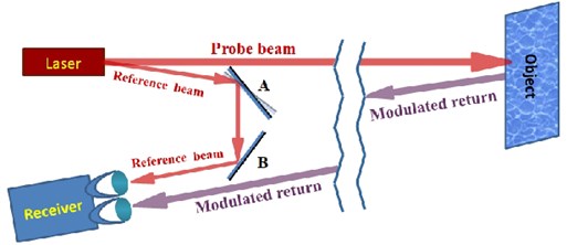
By using a “pencil-thin” beam, conventional laser vibrometry systems can sometimes better identify modes in a simple academic structure such as the solitary vibrating bar in the following photos. However, a large spot size can adequately measure those modes and more. This can be shown by simulation and analytical calculation. The simulation uses FEA for vibration deformation data that is handed-off to a set of MATLAB functions that perform Fresnel propagation for the optical sensing. The FEA shows the mode shapes and calculates the energy per mode which are the modal participation factors (MPFs) [15, 16]. The FEA surface vibration results are input for the MATLAB image propagation calculation (Fresnel propagation [17]). The physical schematic for the simulation appears in Fig. 4. Laser vibrometers use many different methods that can have an effect on the precision of the measurements.
The laboratory measurements of the vibrating bar show the signal to noise ratio (SNR) is quite high for structural components and, unless the system is purposely damped, the resonances are sharp. These sharp resonances lead to the discrete mode picture (stem plot at right in Fig. 1) that the field of modal engineering evolved to exploit. The literature provides the theoretical reasons that strain-energy tends to eschew higher frequency modes and thus populate the lower modes. Years of experience of vehicle design and analysis support these conclusions, as does the FEA of clattering armor plate reported here and in detail in a thesis [7]. The FEA results show that unsymmetrical modes of the clattering plates have higher frequencies than symmetrical (in-phase) vibration of the parallel plates, and that these low frequency modes are discrete below 500 Hz, as is the case with typical automobiles. These modes are usually easy for laser vibrometers to detect. The optical image propagation model shows that even a non-imaging spectrum of the surface of the clattering plates contains energy-ordered modes whose vibration strain-energy drops off with frequency, as described in the Zienkiewicz quotation provided here in Section 3.
Commercial laser vibrometers tend to use pencil-thin spot sizes on the object being measured. This spot's cross-section can be as small as a one pixel response. Large spot size imaging systems have far more information, much of which can help spectral identification (ID), such as the method developed herein. Further, non-imaging signals average responses from all pixels for each time step. An optimum automated target recognition (ATR) system could use a combination of small spot size and full size illumination. But a large spot size tends to help tracking in the paint-the-target phase, while still enhancing spectral ID.
Fig. 4Coherent radiance undergoes a spatially harmonic phase modulation as a function of the probe beam location due to target vehicle surface skin structural vibration. The Object modulates radiance from the outbound probe beam at a distance of up to several kilometers while the receiver system keeps track of the phase of this exitance using the reference beam from articulating beam-splitter A and return mirror B, and appropriate delays (delay fiber or other systems not shown) where appropriate
2. Structural nonlinearities
Several different types of laser vibrometers can measure dynamical properties of vibrating surfaces. The type of laser vibrometer is less important than the phenomenology of what can be measured remotely. A priori project restraints such as requirements to calculate a transfer function, or to use pencil-thin probe beams, can limit the sensed spectra and thus omit or change perceived vehicle behavior(s) in a manner unrelated to errors in measurement or analysis. In many fields such as acoustics, the modal results can be less accurate than a kinematic approach would provide. Nevertheless, especially for complicated nonlinear systems, it sometimes pays to ignore detailed kinematic analysis, which are often invalid for nonlinear systems, in favor of modal engineering to tabulate the modes (deformed shapes for particular resonance frequencies), their frequencies, and their energy or modal participation factors [16].
For over half a century modal engineers routinely used modal analysis for nonlinear vehicle structures. This work uses a structural model of a plate bolted to another plate on a base structure. The work also uses simplified and even “linear” component studies. These studies cannot deliver the behavioral metrics that the full system model provides. Component studies do verify limited aspects of the full nonlinear model, which is a crucial part of the overall analysis. In the full analysis, the structure is a free-floating system using D’Alembert reactions, an analysis technique common to vehicle engineering. See, for example, the numerous “quarter-panel models” in the literature [18, 19], which are mostly meant to show how to model some features for reasons stated previously.
The sensor model is an optical model without the usual air turbulence analysis, except to check for Fante’s wavefront coherence breakup range [20] and a few other imaging issues [7] that are out of the scope of this paper.
The physical model for the clattering armor assumes a linear superposition of vibration modes on a nonlinear structure. This is not a linear time-invariant (LTI) system. The details of removal of these typical LTI assumptions and its relationship to stability, stabilization, and stabilizability, are in the thesis [7], available through DTIC dot mil. The analysis includes a treatment of how changes in fixity causes changes in the modes. Similar changes can model the aging of parts. Therefore, the modulation of the sensed optical radiant flux is related to the analytical nonlinear expressions in the Appendix that help explain the contact nonlinearity in the FEA simulation. The modeling complications related to fixity, nonlinearities, and modal participation factors [15] are dependent on control of the nonlinear solution per time step and over time using load increments, iterations, and other parameters. The analyst also needs to make sure the solution follows the millions of load deflection curves [7, 21] in the full system model.
The finite element analysis (FEA) output represents the three-dimensional structural model of the clattering armor plate system and provides the time history of a structural vibration that modulates the optical return recorded by the sensor. The Appendix contains a set of single and two degree of freedom analyses that result in analytical expressions. The objective of the analyses is to use the optical images, or non-imaging radiant flux (watts), to determine the frequency of structural spectral modes for target identification (ID).
2.1. Modal participation factors
Recent conversations with Navy scientists and engineers tend to evolve into studies of the role that the nature of system observation plays in the perception of the modal system, and how the low frequency strain-energy modes of the structure are effectively quantized. The discrete nature of the modes has been an underlying assumption of modal analysis and in its application to ride-and-handling for half a century. The modal participation factors [16] describe the dynamics of energy flow by using vectors of MPF’s that span the pertinent modes [15]. Each MPF is an element in vectors that are arrays ordered by mode number , used in the FEA of vibrating structures such as vehicles, antennas, and spacecraft. For example, NASTRAN may require ‘DMAP alters’ (macros) to read out some of the components of .
An example of the unintended consequences of design decisions for the 1990 era Corvette follows this detailed restatement of the three modal characteristics introduced earlier, which are essential to the correct system ID. They will be used in the example. (1) The lower frequency modal states (eigenvectors) form discrete modes, even for the complicated system synthesis models and the vehicles they represent. The work of vehicle design for these issues focuses on (2) transition probabilities and (3) the flow of strain-energy that preferentially fills the lower modes with energy, as discussed in the quoted passage in the next section.
2.2. Observational characteristics: discrete, transition, and ordering
1. Discrete modes are countable sets of distinct and high signal to noise ratio (SNR) response of bandwidth narrow enough to be obviously a single mode. The strain-energy levels within each modal state are tabulated by the structural design team in order to determine critical components. These critical regions absorb most of the ride-and-handling and structural engineering effort during vehicle design, resulting in a final list of lower frequency energy levels. The lower modes relate to mode shapes that are usually characteristic of the structure, such as bending, twisting, and stretching. A real-life example appears later in this section.
2. Transitions between modal states, from one eigenvector of the structure to another, are often sigmoid in nature where the region of rapid mode coupling depends on meeting strain-energy thresholds that allow more efficient coupling between modes. Most of the energy tends to flow to components with lower fundamental modes according to characteristic (3) below. Nearly all joints are structurally nonlinear for the transfer of forces and reactions, a situation that provides substantial coupling nonlinearity.
3. Ordering of modal participation: The low frequency end of the spectrum tends to hoard the majority of the strain-energy, as the quote from Zienkiewicz explains. These characteristics are summarized in Table 1, the Conclusion. Analysis of MPF’s (developed by characteristic 2) can determine state transition probabilities. However, modal engineers tend to be focused on solving critical failure issues. Engineers might use similar terms for entirely different kinds of “modes” such as 'failure mode effects analysis’ (FMEA). However, a large part of modal engineering involves creation of a record of the order of the vibration modes, followed by an analysis of the tracks of the modes as the design variables change.
A structural vibration example described below shows how a structural design change can de-couple modes in order to improve ride-and-handling. However, this change has consequences other than aesthetic design constraints. The changes can increase crashworthiness risk and other seemingly unrelated systems, and they can degrade previously adequate vibration and modal engineering balances in the design. For example, stiffening one joint or component usually provides a much more efficient flow of energy through that stiffened element of the structure. Strain-energy is drawn from the high frequency modes to the low modes in a surprisingly efficient manner once such a structural “channel” is open (components have structural coherence). Then the MPF’s start to re-balance as the entire integrated structure starts to equilibrate. So a stiffener can solve one problem and cause another. The engineering group that deals with braking and crash loads that transfer from the front to rear bumper can have its margins go from adequate to negative due to a design change by the ride-and-handling team that solves a mode-coupling problem. This is similar to an old solution to convertible mode coupling:
2.3. Inter-organizational effects of design changes
The 1980 era Chevrolet Corvette convertibles initial design had a fundamental bending mode just below 30 Hz, which put it very close to the suspension mode. This is an overall vehicle bending mode that curves about a lateral axis, where the bumpers move vertically and together, both in direct opposition to the vertical motion of the seats. It is usually the lowest frequency vehicle mode for a convertible (as if the vehicle is trying to do sit-ups). The Corvette designers needed to stiffen this mode to reduce coupling to the nearby suspension modes, which were also near 30 Hz. The models in the late 1980’s had very tall rockers that satisfied this requirement. This was the most efficient structural fix because the stiffness of a beam to bending vertically is proportional to the cube of its section height [26]. Apart from the aesthetic issue with having to step high to get into the Corvette, these tall rockers also changed other load paths including a for-aft transmission of load, important to crashworthiness, as well as making the vehicle slightly more heavy. Automotive is one of the few industries that has a price on the engineering sufficient to remove a kilogram of mass, which was $50,000 in 1990. These and other costs were accepted in order to move the fundamental bending mode away from the suspension mode to effectively eliminate coupling. In later years, other technologies helped solve this issue.
With the exception of the Pininfarina chassis test results [12], few modal analyses such as these (chassis or body-in-white) are in the literature. To a scientist, the ride-and-handling issues and how they relate to the three observational characteristics described above might seem to be basic enough to warrant several scholarly articles. However, this is clearly the arena of trade secrecy at such a high level of value that corporate lawyers would be unsurprised at the paucity of measured data available to the public.
2.4. Measured data: vibrating clamped-clamped bar
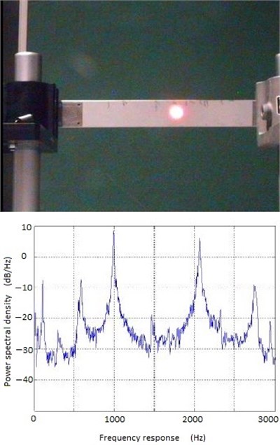
In his thesis Fl. Lt. Ngoya Pepela (he was an Australian Flight Lieutenant in 2006) showed that the modes are not just maxima of a spectrum, but spikes with huge SNRs in the spectral response [10]. These are the “discrete” modes described above in Observation 1. His Figs. 5 and 6 each show a photo of the vibrating bar illuminated by a laser vibrometer, with the corresponding spectral density plot are beneath the photos, plotted in the lower pane of each figure. The first (Fig. 5) shows all the major modes whereas the second (Fig. 6) is missing the modes at 1460 Hz. In Fig. 6 the vibrating bar is seen to be illuminated by a laser beam with a large round spot size centered on the 1460 Hz node of the vibrating bar. In Fig. 5 the right half of the laser beam of Fig. 6 is blocked, illuminating only the left half of the symmetric 1460 Hz mode shape. The halved beam size (Fig. 5) allows the laser vibrometry spectral analysis system to show a stronger 1460 Hz mode return due to the elimination of spatial averaging. That averaging is introduce by phase-related destructive interference from both sides of the 1460 Hz mode shape in the full spot size result of Fig. 5.
Fig. 5The image from a small spot size makes a spectrum with a f3 = 1460 Hz mode. Permission N. Pepela [10, 27]
![The image from a small spot size makes a spectrum with a f3 = 1460 Hz mode. Permission N. Pepela [10, 27]](https://static-01.extrica.com/articles/20501/20501-img5.jpg)
Fig. 6A larger laser spot size creates a laser vibrometry spectrum where the f3 = 1460 Hz mode phase-averages away
Initially spectral elimination might appear to be a problem for the laser vibrometry industry for use with non-imaging sensors if the spot size is large. However, Ngoya Pepela’s thesis [10] and another article by the author [27], with support from simulation and analytical calculations, show numerically how unlikely spectral elimination is for commonly manufactured items, even if the spot size encompasses the entire vehicle. Furthermore, it is necessary, but not sufficient that super-symmetric structures produce spectral elimination in laser vibrometry [7]. The vibrating bar is the simplest form of structural super-symmetry that results in spectral elimination, but it is rarely the only structural component a laser vibrometer can use for identification of a manufactured structural system (vehicle), unless the target is the vibrating bar (a structural oscillator) that requires identification. But even for such oscillators, the typical transducer is a piezoelectric system that is not super-symmetric, and thus not prone to spectral elimination; the source of oscillator energy is separate from the driven bar. Therefore, a vehicle that is purposefully fitted with vibrating bars can still be identified with its spectral “fingerprint” in spite of possible spectral elimination from oscillators. Pepela’s result [10] was that use of small spot sizes reduces spectral elimination from the laser vibrometry spectral result (Fig. 6 vice 5).
2.5. The McKinley observation
In early 2018 Michael McKinley of Arlington, Texas, observed that Fig. 6 contains modes (at approximately 2740 and 2900 hertz) that are not visible in the small spot size collection [28] in Fig. 5. While the small spot size is still large enough to average out higher frequency (smaller vibration shape wavelength) modes, another spectral elimination that small spot size vibrometers are susceptible to is the effect of the probe spot being on a Chladni line of nodes [29] of the vibration shape for particular frequencies [30]. Detection of these modes at 2300, 2740, and 2900 Hz is a positive observational difference provided by using a large spot size, in this case.
Therefore, spectral reduction and elimination (SR and SE) happens for all spot sizes, large and small, for super-symmetric structures such as 1-D bars. The prior paragraph discusses why this is not a problem for manufactured vehicles; nature provides a mitigation (vibrometry is a useful classifier system for realizable structures) of the perceived problem that the McKinley observation clarifies (small spot sizes do not mitigate SE).
2.6. Observational differences
The difference between small spot size (Fig. 5), and larger spot size (Fig. 6) comprises one dimension of observation variation that can change the observer’s view of reality. Physical systems such as the Corvette design example can be used to explain the existence of the three characteristics of modal systems listed above. Contact nonlinearity is the main physical model of interest in this paper because contact is a relatively simple and ubiquitous form of nonlinearity, found in nearly all structural joints.
3. Energy ordering
Vibration strain-energy transfers from one component to another, usually through joints that are necessarily nonlinear (even spot welds), depending on the amount of “fixity” of that interface or joint. An extensive treatment of how fixity changes the modes and therefore the sensed optical radiant flux is in the author’s thesis [7, B.2.3, p. 187], including nonlinear examples that compare to the contact nonlinearity of the FE model. Fixity is an engineering variable for a particular DOF that determines the ratio from zero to one (0 % to 100 %) of force, moment, or torsion [26] that will transfer from one component to another through the joint member for whom the fixity is defined [25].
Even “simple” vehicle structures have complicated load paths that are nonlinear (mostly through joints) where forces from one region of the vehicle affect parts elsewhere on the vehicle. These are the pathways for vibration energy flow that tend to dump energy into low frequency structural modes. Modal engineers use isolators and suppressors to stymie this natural tendency, but mostly just for critical components. Some components tend to have non-negligible vibration spectral energy down at these “fundamental” and near fundamental modes even without the nonlinear effects. Damping helps drive the energy into the lowest modes because the resonance spreads (widens) to encompass a larger bandwidth.
Zienkiewicz showed energy transfer using only viscous damping [21, p. 340-341] to form a ratio of damping to its critical value, depending on the modal frequency , as quoted below. For vibration systems that are driven by a forcing function , Zienkiewicz describes the differential equation (DE) using a mass matrix (), a damping matrix (), and a stiffness matrix (), acting on deflection and force vectors and . and are damping parameters.
Zienkiewicz quote: “... we have indicated that the damping matrix is often assumed as . Indeed a form of this type is necessary for the use of modal decomposition, although other generalizations are possible [references given in the book]. From the definition of , the critical damping ratio [described above], we see that this can now be written as:
Thus, if the coefficient is of larger importance, as is the case with most structural damping, grows with and at high frequency an over-damped condition will arise. This is indeed fortunate as, in general, an infinite number of high frequencies exist which are not modeled by any finite element discretizations.” [21, p. 340-341]
Therefore, vibrational strain-energy tends to naturally migrate from higher to lower frequency modes. Some of the strain-energy can find its way down to the lower modes because over-damping causes more overlap of modal response resonances. Nonlinearities add to the methods of energy transport as discussed later.
This results in a set of modes where the mode number increases monotonically with frequency and has an energy that decreases monotonically with mode number. Possible exceptions to this natural effect include artificial structures or temporary transients such as might be introduced with magneto-rheological fluid or other systems controlled by magnetic or electric field variations. The 1/ phenomenon is found in many different fields of engineering.
The local mode structure in Ngoya Pepela’s laboratory test measurement in Figs. 5 and 6, which do not follow the 1/ phenomenon within the displayed 3 kHz, appears to be a contrary example. This is an example of not being able to “see the trees for the forest” within its part of the response spectrum of the very stiff clamped-clamped structure. For those results, the vibrating bar only had a half-dozen distinct modes across 0-3000 Hz, one of which was diminished in Fig. 6. The utility of the structurally super-symmetric bar is that it shows discrete modes, and that the energy in some modes is spectrally reduced or eliminated by spatial “averaging” – integration over the area of a surface of variable phase that introduces varying levels of continuous interference depending in large part on the limits of spatial integration [27].
That the vibrating bar of Figs. 5 and 6 is consistent with modal ordering becomes apparent by analysis of the physics of a simple model of a point mass at the end of a spring of stiffness . This explanation considers multi-variate non-uniform parametric change in the system. The maximum potential energy is approximately where is the largest extension of a simple spring. Assume that the frequency is increased, then the energy grows as the square of the frequency, parabolically as . In practice, the deflection decreases with frequency, as it must. However, there is a practical limit to reduction in deflection. When that limit is reached, while the frequency continues to increase, the potential energy must grow. This means that higher frequency modes require more energy, even for smaller deflection – especially when deflection is already small, when . The kinetic energy side of this simple calculation is Rayleigh’s method [31].
It may help to see this from a force point of view using the gradient of . If the restoring force is conservative, it is , and is thus a quadratic function of the frequency, . It might be tempting to consider a “conjugate force” for frequency, where the gradient (units of action: Energy × time, or momentum × distance) [32]. However, the force (), cannot increase ad infinitum with . At some point assumptions of linearity and structural integrity start breaking down. Combining the observations of this upper limit on the force, and the understanding that the spring extension is limited to , the energy required to have a particular mode increases approximately quadratically with . This increase strain energy based on the modal displacement is “on average” energy in this sense – that the other variables are limited, and using experience that dynamical systems naturally tend to avoid populating the higher modes with energy. Many children experience this effect when they try to forcefully excite a higher frequency mode in a rope, only to fail unless they exert considerable effort to the point of overexertion.
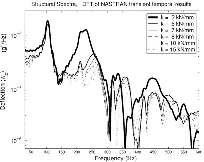
Using the observations above, a conjecture can be stated for the system restoring force of simple harmonic motion, based on the gradient of potential energy, along with the FEA simulation included herein (Fig. 7), including industrial experience, and the test data from the childhood of most of us. While system energy decays with frequency “on average”, a plot of the spectrum within its lowest half dozen modes might not show the 1/ phenomenon, but that the full pattern does. Sometimes the spectrum plot is “in the trees” and the “forest” of the 1/ phenomenon over the entire large bandwidth spectrum is not seen within the zoomed-in window of smaller width. For example, consider the “in the trees” ranges of 150-250 Hz and 400-500 Hz for the much lower fundamental frequency system of clattering armor in the FEA results of Fig. 7.
This figure plots several spectra of the simulated structure, 1×2 meter clattering plate (homogeneous rolled armor, discussed later). There is one curve for each level of damping (see legend) and they show a different method of inter-modal energy transport. The 1/ pattern shows up in its structural vibration spectrum. A collection of the deformed shapes for transient analysis in the CSC thesis [7] shows how the transient result at each time step is a superposition of normal modes (eigenvectors) populated with energy according to the MPFs . Those normal modes plots show how one mode at one frequency for one plate excites another mode at a different frequency on the other plate because of deflections that line up along the surface to contact the other plate at anti-nodes of a different mode. Again, the lower modes tend to be receiving modes.
Using appropriate structural damping, the frequency response function in Fig. 7 is the result of an impulse load that rings all the modes of the FE model. It appears to be natural that MPFs decrease with the mode number of the mode they characterize; in a time-averaged sense, the vector is an array of monotonically decreasing participation values usually measured as the strain-energy for each mode. This is part of the reason for the ubiquitous 1/ phenomenon. At least for structural vibration [33], we can thank the Zienkiewicz section quoted above [21, p. 340-341] for providing an explanation of at least some of this 1/ fall-off.
Fig. 7Spectra for armor-hull clattering systems, except for the symmetrical modes. Results use different armor-hull baffle stiffnesses (see legend)
4. Simple harmonic motion, not so simple
A spring-damper-mass single DOF system (SDOF) provides a one dimensional model of the clattering armor plate which can provide analytical solutions to the vibration DEs. Assume “small deflection”, where strain-energy density is low enough for linear elasticity assumptions (lack of permanent set in the structure being modeled). Also assume that modes are nearly monochromatic functions of sines and cosines.
In a more formal development of the transfer of energy from one mode to another, Lord Rayleigh points out that pure sine or cosine waves do not exist in reality. He derived the differential equations for Newton’s theory for isothermal compressive-vacuum vibration resulting in this second order form [16]. The footnote describes these generic variables in Eq. (1) for a wave in with respect to and time . These concepts are covered in engineering vibration textbooks [29, p. 30]:
Lord Rayleigh then comments on the ability of simple harmonic motion to maintain shape in nature. The extent to which the mode shapes are not harmonic introduces a possible corruption of the pure energy-per-mode concept assumed by MPFs. In the scientific literature a “mode” is derived from the parameters used for the study of statistics which include the median, mean, and the mode. In a field where Gaussian distributions abound thanks to the physics described by the Central Limit Theorem, the mode is merely the location on the abscissa, in terms of the frequency for a spectrum, at the maximum of the response. In this sense the typical emphasis on energy-in-mode used by modal engineers is appropriate [22] to identify the deformed shape of the eigenvector for that approximate center frequency. However, transfer functions are inappropriate for these nonlinear systems. If transfer functions are modified as Bendat does for simple solitary nonlinear systems [14], which is out of the scope of this work, there may be some consistency between the methods that would be useful to develop, separately.
4.1. Contact nonlinear response
The author's CSC thesis [7, App F] describes and plots the control law as a sigmoid for the stiffness, which is the slope of the load-deflection curve. The control law is a mathematical representation of the nonlinear stiffness associated with the contact state between armor and hull. This classifier is an arctangent function, a smooth version of the typical bilinear gap element load-deflection table. As the armor and hull make and break contact, the stiffness switches between high and low values of stiffness, respectively. When the armor and hull are in contact, negative deflection (compressive penetration) results and there is a large stiffness due to the large slope of the deflection curve. When the armor has separated from the hull, the nonlinear contact stiffness becomes a deflection curve of small slope. This small value of extra stiffness provides computational stability. The author's thesis [7] contains a description of the stability and application of the control law for this case, demonstrating that the damping DOF and frequency DOFs are no longer related. The following analysis expands on one of Dr. Winthrop’s control laws listed in his 2004 AFIT dissertation [39]. His is a different control law, but the analysis methods are complementary.
Phase space (state space) plots [7, Fig. 12] validate this model’s behavior. The arctangent function that does the switching in this simple closed form model appears in state space formulation as shown below in Eq. (2), which has the constants listed as Eq. (3). The state space description for the single mass speed, , and acceleration, , shown in Eq. (2) is a function of the open and closed stiffnesses, and , for a damping coefficient of in units of hertz, where is a point mass:
This model of a “welded-together” panel system uses the parameters in Eq. (3). A “manual”, analytical calculation [7, App C] helped validate the FEA results for the simulated vibration created before application of the laser vibrometry model. Ngoya Pepela’s optically measured modes provided qualitative support for the application of the laser vibrometry model that used the FEA results to modulate the probe beam. This section and the Appendix describes the former, a structural SDOF model:
In the arctangent gap model [7, Fig. 11] (not plotted here), the stiffness will transition at contact, . Contact surfaces are imperfect due to microscopic protuberances that comprise the roughness of the surfaces. As the two plates come into contact () the roughness of the surfaces deform, compressing the protuberances, and a transition from low to high stiffness occurs rapidly in order to match the surrounding material. For a “low” damping system, the damping is 0.02 kg/s and the open to closed dimensionless stiffness ratio is 0.01. The Appendix describes the dimensioned and dimensionless models. A plot of speed versus gap opening in the thesis [7, Fig. 12] reveals that the high stiffness during compression of the base is a shallow orbit in versus phase space. Changes in damping lead to changes in the range of the orbits during stabilization. These control law formulations were implemented using a MATLAB system [40].
Lyapunov function analysis shows the contact control law is asymptotically stable. The Lyapunov function in this case is the total energy with simple damping loss. In rare cases vibration energy gain to the hull upon which the armor plate clatters matches the cycle’s damping energy losses and is in synch with plate contact. Persistent energy loss is due to structural damping, material heat losses due to bending, and fastener frictional losses. The energy gain per cycle is less than the energy loss due to damping [7, App F]. If the losses were small enough to just equal the gains, the system would be “stable in the sense of Lyapunov”.
This analysis above summarizes a clattering system. Details of the physics of boundary conditions, initial conditions, and operating states are found in the thesis [7, App F].
4.2. Laser vibrometry return from the probe beam
The noise floor did not rise in Fig. 6, but rather the surrounding spatial areas had phase differences within the large spot size that, due to spatial averaging, underwent destructive interference in a bandwidth that removed most of the 1460 hertz mode. This interference is a combination of optical phase shifts along-range caused by reflection from deflection amplitudes that are related to the structural wavelength along the bar for each mode.
The purpose of the vibrating bar measurement was to show spectral elimination, but it also shows the discrete nature of high quality (low damping) structural modes. The FEA of this system [7] complemented this laboratory measurement [10] by showing that, while spectral elimination can occur with structures that might be constructed in the lab (one dimensional modes shapes are the simplest super-symmetric structures), it is impractical to build commercial structures that are substantially super-symmetric.
The main result of the CSC simulations was that academic models can produce reductions of vibration sensitivity that theoretically verify part of Ngoya Pepela’s spectral elimination thesis [10], within meaningful assumptions. The single and two DOF models described here show why this is the case, theoretically. A separate 2014 article [27] describes the lack of spectral elimination (or spectral reduction) for vehicle and other types of structures that are manufactured economically.
The lab vibration measurement shared some spectral reduction features seen in the nonlinear cross-spectral covariance simulation [7]. The transient vibration results for the surface of the 3-D armor plate were the input for a MATLAB system that forms an image similar to one that a laser vibrometer would detect. Commercial laser vibrometers typically only provide images processed with their proprietary system. For the purpose of simulating the image of the vibrating plate, the optical model for this work used conventional Fresnel diffraction in a MATLAB system of functions. The Fresnel propagation method introduced by Goodman [17] provides a computationally adequate method to propagate an image of the return from the target back to the detector. In this sense, Pepela’s laboratory measurement provided a validation for the FEA and vice versa.
The laboratory measurements in Figs. 5 and 6 use a clamped-clamped bar that has a high frequency fundamental mode (compared to vehicle fundamental modes that are below 50 Hz). The spectrum has not dropped off with frequency by 3 kHz because this is still the “lower frequency region” for the structure, as discussed in the Section 3. It has a stiff fixity meant to test the laser vibrometer for structural wavelengths that would undergo a difference in phase across the beam spot size.
The spectral elimination effect, seen mostly in (Fig. 6), provided laser vibrometer manufacturers information on what spot size to suggest or program for their probe beams. They want to avoid such “spectral elimination”. The simulation and analysis in the CSC thesis [7] shows users and manufacturers that, except for 1-D structures (bars), even specially manufactured structures are difficult to create in the super-symmetric form, and thus do not exhibit spectral elimination.
A detailed study is available that has comparisons of both structural and optically sensed CSCs, to imaging versus non-imaging returns [7]. The latter choice of observation type, non-imaging, analyzes a scalar signal composed of the spatial average of the entire image per time step. The simulation analyzes the surface of homogeneous rolled armor (HRA) using only one scalar metric, radiant flux that is the spatial integration of the irradiance reflected from the HRA. These coupled FEA-optics results, using non-imaging return, identify the modes on the target (HRA clattering on a hull), nearly as well as the imaging version of the CSC.
4.3. Finite element modeling and analysis
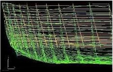
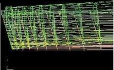
The FEA produces a surface of vibration that is curved in 3-D. The vibrational deflections are the input for the scripts and functions run within MATLAB that produce an optical simulation of the target’s image. Unlike the small and large spot sizes (Figs. 5 and 6) in Ngoya Pepela’s measurement [10], the remote sensing of the armor-plate clattering uses a complete coverage large spot size such that all points on the armor modulate the probe beam. Assume the surrounding clutter to be time-gated or otherwise removed. The input that the MATLAB script uses is the set of displacements to simulate images of the transient dynamical response of the surface of the clattering armor for hundreds of time steps in a duration of a few seconds. One such “vibration deformed shape” is seen in Fig. 8.
Fig. 8FEA of the deformed shape (green) for the clattering armor-on-hull model. Exaggerated micron deflections would not be visible compared to the large physical geometry of the plates. There is a 14.24 ms time difference (many time steps) between these two output time frames. The views are into the fore-shortened long direction (1 m) of the 0.5 m wide plate. The un-deformed shape is a light tan color
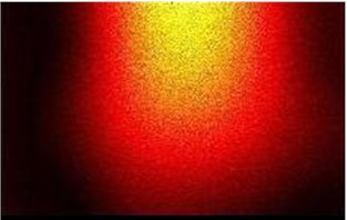
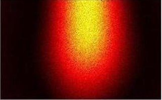
The FEA representation of the vibration shape was applied to the MATLAB model of the probe beam as a phase modulation. Using Fresnel diffraction [17], the return was imaged onto the detector 4 km away. A 10 μm probe wavelength satisfied the numerical requirements for results shown in Fig. 9.
A spectrum of the time sequence of sensed images, such as the two shown in Fig. 9, appears in Fig. 8. More detailed plots are available [7].
Fig. 9Simulated magnitude of radiant flux image of the return after modulation by the vibrating plate in Fig. 8. The image horizontal width appears rotated 90 degrees from the long fore-shortened axis in the prior image in order to better display the 20×40 mm detector grid shape. The maximum deflection “hill” along the 1 m length shows up as a vertical maximum magnitude in the lower (later) pane of both figures
5. Nonlinear eigen-states
Creating a simple model for a clattering structure may seem easy, until the fact that the eigenvalues must be nonlinear complex functions becomes apparent. A two degree of freedom (DoF) model developed in the Appendix herein was meant to validate the FEA. This FEA validates a major dynamical 2 DOF analysis result: Antisymmetrical and unsymmetrical modes increase in frequency for increases in contact stiffness. Investigation of these closed form simple damped sprung mass systems provides not only insight, but qualitative numerical validation as to whether an eigenvalue increases for antisymmetric and un-symmetrical modes as gap-closed stiffness increases. This simple model result provides another analytical basis for results seen in the FEA. Additionally, the behavior of the modes indicates that symmetrical modes are better target identification features than un-symmetrical modes. Hence, there is a need to analyze the energy balance and stability [7, App F] to validate the simple one and two DOF models as is summarized in the Appendix herein, including the time variation of amplitude and phase.
Using the SDOF model as a basis, the Appendix uses Eq. (4) to provide the 2DOF solution. Eq. (4) may appear deceptively simple because the time variation of the amplitude and phase is not apparent until explicitly formed. Eigenvalues are complicated functions of natural frequencies of individual modes which require “mode tracking” [41] with respect to stiffnesses [42], due to their transient nature in reality [43]. Fig. 10 plots the real part of the dimensionless eigenvalues of Eq. (4) as a function of dimensionless frequency versus dimensionless closed stiffness , scaled by the hull stiffness for a closed stiffness [7]. Two models appear in Fig. 10. The hull system is eight times stiffer than the “armor” system:
Fig. 10Real parts of the eigenvalues for the dimensionless DE show why higher-energy antisymmetric modes are less likely to be excited. Above a k crit the symmetric (lower frequency branch) and antisymmetric (higher frequency branch) modes [29, p. 167] for this two DOF problem break out into modes of well separated energy
![Real parts of the eigenvalues for the dimensionless DE show why higher-energy antisymmetric modes are less likely to be excited. Above a k crit the symmetric (lower frequency branch) and antisymmetric (higher frequency branch) modes [29, p. 167] for this two DOF problem break out into modes of well separated energy](https://static-01.extrica.com/articles/20501/20501-img12.jpg)
From a chaos point of view, nonlinear attractors exist for the system defined by Eq. (4). We know this because the systems exist in reality and their vibration modes do fluctuate, albeit not monotonically. The nonlinear attractors are related to the underlying hull forcing functions (D’Alambert’s forces due to vehicle inertial loads), the timing and shape of the clattering, the plate stiffnesses, the structural and added damping (e.g., washers or armor-hull batting), and the fixity of the joints.
Initially the two eigenvalues for the 2DOF system are equal. As the closed stiffness increases, a critical value of stiffness, , is reached where the armor can no longer follow the hull. It starts to clatter in an unsymmetrical mode. A 3-D contact surface cannot be anti-symmetric unless it is axisymmetric (1-D), as are the SDOF and 2DOF models. When the stiffness exceeds the two curves become distinct, branching into two separate paths. This can be see for the plots of two models where the base stiffness is 128 and 1024 N/mm. In the region before clattering, the slope of the 8× higher base stiffness curve is one eighth of the slope of the smaller base stiffness curve. At this higher 1024 N/mm base stiffness there is also an eight-fold increase in . The intercept also increases 8-fold. Derivations of these concepts and further results, including how the imaginary parts of the frequencies (not shown, Fig. 10 is the real part) contribute to the transfer of energy between the modes are developed in the Appendix.
6. Analysis and conclusion
A system model of the structural vibration of a contact-plate system was shown to have surface waves with low frequency modes that are effectively discrete modes of the PSD [17]. This clattering armor system provided an example of nonlinear response. Both SDOF and 2DOF models derived in the Appendix have qualitatively verified the symmetrical versus unsymmetrical modes, and the higher frequency of the unsymmetrical clattering modes. The full finite element model transient results also showed the tendency for vibration strain-energy to collect in the lower frequency modes, as most model engineers have seen [12], and as was calculated analytically in the classical literature [21, p. 340-341].
(1) The lab tests on the doubly clamped bar show experimentally that high SNR modes are effectively discrete. In the absence of substantial damping they are not just the maxima of a spectrum, but spikes in the spectral response [10]. The system in Fig. 5 has a signal-to-noise-ratio that is huge. These massive SNRs show that the lower modes of structure, that are fairly high in frequency for this case due to the double clamped nature of the bar, can easily be considered discrete. Hence, quoderat demonstrandum (Q.E.D.), the observational characteristic (1) is demonstrated – lower frequency modes are essentially discrete.
This analysis of nonlinear eigenvalues provides useful results for theory and simulation for common nonlinear structures. Symmetrically moving parallel plates have more strain (and thus more strain-energy) than clattering plates where the unsymmetrical motion interrupts their nearly sinusoidal in time out-of-plane-motion to spew strain-energy into acoustics and even permanent set (deformation of the material). Through simulation and by experience the observational characteristic (1) appears true, that lower modes are effectively discrete for high quality systems (low damping), and that, when there are pathways (nonlinear joints) that allow energy transfer, (2) and (3) are in effect; damping and clattering help the energy flow into the lower modes from higher frequency modes – although overall energy is lower as damping increases (see Fig. 7). Most vehicle components have bolted or riveted joints that allow such energy transfer [16] as can be seen with plots of coherence spectra, [44].
Table 1Comparison of observational characteristics related to spectral elimination (SE)
Characteristic | Discrete modes | Energy transitions | Energy ordered by mode |
Concept sketches | Fig. 1 () | Fig. 2 () | Fig. 3 () |
Dependency | High resonances | Clattering FEA model | Same deflection at high frequencies |
Spectral effect | Figs. 5 and 6 | Fig. 7 | Damping, eschews [21] |
Character | Low frequency | Nonlinear joints | Steady state vibration energy |
Small spot size | Sees all modes | Blind to many | No Spectral elimination (SE) |
Large probe spot | SE in bars | Sees more | Some SE (spectral reduction) |
Super-symmetric | Some missed modes | Misses most | Provides th. of SE [27]. Target rarely super-sym. |
Manufactured parts | Sees all modes, Fig. 7 | FRF, , MPFs | Typ. Fig. 7 (super-sym. target is rare) |
(2) The tools in industry that provide MPFs include mature engineering methods [16] from the 1980's such as the FEA tools put in place, for example, by MacNeal-Schwendler Corporation engineers in NASTRAN [15]. These MPFs stored in the FEA vector can measure the energy transmitted between states (between eigenvectors of the system) where the state (mode) changes its energy with mode . . For surface waves on the ocean [45] this observation would include wave energy of large ocean swells driving up capillary waves and eventually creating foam as seen in large storms. Energy transfers from one type of wave to another, Rossby-Kelvin, gravity-capillary, internal-surface, ..., and direction variations thereof, may prove useful.
Modal engineering for industry, especially for vehicles (i.e., ride-and-handling) is a trade secret endeavor. Vibration spectral plots for vehicles found in the literature, such as the Pininfarina paper [12] are rare. It makes use of analysis tools in order to calculate modal participation factors [15]. These MPFs show the “participation” (energy per mode [16]) using modes developed from normal modes that are FEA-produced eigenvectors. The participation flows from energetic modes to lower energy modes is similar to how large swells on the ocean in a storm are accompanied by unsettled surfaces, rather than smooth large waves that a tsunami has before it nears the shore [46]. In the latter case, not enough time has passed to transfer the energy to other modes until the wave crashes on shore where sufficient coupling to other modes exists due to the constraints of the shore structures.
Therefore, due to (3) the energy ordering of modal states for complicated system synthesis models and the ordinary vehicles they represent, the work of vehicle design for these issues focuses on (2) transition probabilities and (1) energy levels . There are usually other types of oscillator interactions that produce an ordering of energy levels similar to that described by Zienkiewicz [21, p. 340-341]. These concepts are summarized in Table 1.
Pencil-thin probe beams like that used in the lab measurement have observational characteristics quite different from the large spot size used for the FEA-MATLAB model of fully illuminated clattering armor. The former can be less susceptible to spectral elimination. However, Mr. McKinley’s observations discussed in section 2.4 on page 6 show different modes appear and disappear for either change in spot size. The latter low fidelity beam method is adequate for spectral identification of economically manufactured vehicles. Such full coverage probe beams are less likely to be subject to spatial coherence issues or illuminate solely a node of the Chladni zone [30]. Pencil-thin beam returns fail to convey vibration modulation in this manner [29]. For the large (full coverage) spot size, some of the beam will nearly always get through.
While these results are generic for plate structures, application to waves on the surface of a volume appear to fulfill similar behavior of (1) discrete modes, (2) modal participation dissipation, and (3) higher energy in lower frequency modes. A tsunami distant from the littoral shallows has a much lower spatial frequency and temporal frequency than typical 2-4 meter gravity waves. However, the larger Rossby and Kelvin waves are also candidates for the study of the extreme low frequency application of the principles observed in this article.
7. Appendix – one and two DOF contact eigenvalues
This Appendix summarizes the nonlinear dynamics of simplified 1-D and 2-D forms of a structural contact system, its relationship to the full 3-D FEA, and in the end, test measurements. The 2-D form provides for a difference in foundation stiffness, and transition to 3-D.
7.1. Closed-form SDOF nonlinear contact response
This subsection displays the Mathcad output for the closed form solution to the damped SDOF oscillator meant to represent a lumped mass model of the HRA-hull contact vibration system. The mathematical derivations are based on the nonlinear solutions [39] with a simplification of the control law, , that models simple contact along the -axis.
The SDOF dimensionless system describes the effect of nonlinear contact stiffness from a solution composed of symmetric and antisymmetric one dimensional modes. This SDOF solution applies to the symmetrical and unsymmetrical modes of the 3-D FE model for the HRA-hull system, respectively. In 3-D the unsymmetrical modes are non-uniform, occurring when some parts of the armor is moving opposite to the hull (i.e. clattering). For clarity 1-D modes are distinguished as symmetric or antisymmetric, while 3-D systems are labeled symmetrical and unsymmetrical. Application of derivatives to the dimensionless system is first made under the assumption that all variables are nonlinear functions of time. Then after starting with a restricted case, the variables are brought into explicit nonlinear use, one at a time, to refine the calculation.
The state-space representation [47] is shown here in its phase space form (location and derivatives). With the definition :
Even the first derivative of Eq. (5), is non-trivial. Mathcad allows factoring in several ways. Collecting on and then on , Eq. (6) provides a compact expression for the undamped speed:
With more assumptions restricting the nonlinearity of the solution where appropriate, the acceleration is also collected on and then in Eq. (7) for this simplified expression:
The first order nonlinear solution in Eq. (7) uses a constant amplitude, constant. While not explicitly a function of time, has a constant time rate of change, . A further order of nonlinearity to allow the amplitude change rate to be a function of time would follow the above assumption with the use of , the time rate of change of a dimensionless frequency. The following subsections describe how Fig. 10 shows that while the stabilizing stiffness increases above the critical lift-off frequency, symmetric modes remain at a constant frequency while antisymmetric modes increase in frequency. This 1-D behavior implies the same effect for 3-D modes, symmetrical and unsymmetrical, as is seen in the FEA results [7].
7.2. Closed-form Mathcad 2 DOF contact
Mathcad symbolic equations in the following calculations comprise the closed form solutions for a damped two DOF (2DOF) contact vibration model. Stiffness is the “rate” that represents the sharpness (hardness) of the contact.
7.3. Two DOF DE’s and solutions
Eq. (8) is a dimensioned form of the two DOF damped oscillator DE where , , , , , , and are applied force, outboard mass, foundation stiffness, damping, control law stiffness, surface displacement, and time:
The dimensionless ratio is the stiffness from the second oscillating point mass (the 1-D representation of the armor) to the base of the system as a whole, which includes the hull for this SDOF system. The hull is freed to oscillate in the 2DOF system. The dimensioned variable is the gap opening in the dimensionless x direction. The dimensioned control law for structural contact for this two DOF problem is the displacement of Eq. (9). The dimensionless stiffness from the first oscillator to ground is unity.
indicates the dimensioned form of gap opening in the dimensionless direction. The dimensioned control law for structural contact for this two DOF problem is the displacement of Eq. (9):
The use of Winthrop’s method [39] on Eq. (8) produces the dimensionless DE in Eq. (10). The dimensionless applied load is and the dimensionless stiffness only applies to DOF one: :
Eq. (11) uses the vector , the dimensionless location of the two masses where is the gap opening. Continuing with Winthrop's assumptions [39] assumes a straightforward solution. Eq. (11) shows all the variables that vary with time:
Substituting assumed solutions from Eq. (11) into Eq. (10) results in a Special Eigenvalue Problem (SEVP). The dimensionless system frequencies are functions of the individual frequencies from where from Eq. (8). Two assumptions help make the solutions tractable. First, the removal of the driving load provides the homogeneous solution. Second, variables dependent on time and space (uniformity with respect to location) vary differently. To first order the time variation of the dimensionless frequency, , is the derivative in this nonlinear system that has the largest effect on the solution [39]. Eq. (12) summaries some of the simplifications:
In words, these simplifications are:
• Constant amplitude, , cancels out of the DE.
• Uniform damping, , is for simplicity.
• But uniform phase, , is realistic.
• Solve for free vibration first (homogeneous solution)
Using a new variable for dimensionless phase, , to simplify the state space gap opening (Eq. (5) simplified in Eq. (11)), the solution starts with a definition of the speed Eq. (13) and acceleration Eq. (14), where coefficients are maintained as variables of time in the derivatives:
Maintain the coefficients as variables of time in the subsequent derivative:
Using Eqs. (13, 14), time derivatives formed below come from application of these differential operators:
From Eq. (10) the resulting dimensionless DE in Eq. (16) below starts to take the form of an SEVP Eq. (17), easily solved by eigenvalue methods. The time derivative operators and (defined above) allow the vector to factor out. The damping constant, , and dimensionless frequency, , remain in the calculation until the “nonlinear” eigenvalues and eigenvectors are developed in the formal SEVP solution. A purely imaginary frequency is in the exponential term in where the sign of indicates damping. The ensuing 1-D analysis provides insight into the dynamics and validates the transient “nonlinear” modes output by the 3-D FEA, modes that exist in reality:
These relations use a different dimensionless stiffness, where and for numerical stability. Eq. (16) is of the SEVP format as shown below in Eq. (17):
Eq. (18) shows the format of the system matrix for submission to an eigen-solver. Some of the terms in and were kind enough to cancel:
Solution of the characteristic polynomial, , provides the eigenvalues of the system where both DOF have equal displacements. Using a Mathcad’97 symbolic solver two solutions are available: (1) Free classical vibration, and (2) a “welded” system vibration solution. The latter welded components (the two masses) is equivalent to being epoxied with hard rubber [7]. As defined in Eq. (9), the welded model reduces to free vibration for slight contact, = 0, just before compression when turns negative. The system dynamics are revealed via the welded solution as the control law is varied in the range . The switching control law, , determines which frequency is active, switching from one frequency value for the open gap state to another for closed gap state. The nonlinear FEA results for 3-D show that both modes are active at the same time at different locations on the surface. Spectral energy flows into and out of both “open gap” and “closed gap” modes when averaged over many cycles of time. The contact gap system is a time composite system with dynamics that are more easily modeled using modal analysis techniques. The noise and vibration industry developed these techniques with nonlinearities such as contact in mind [23, 50-52].
States evolve in an oscillatory manner. This energy flow between alternately created and destroyed states might be a useful model for other systems where the physics appears to forbid continuous energy level ordering. For vehicle structures, experience indicates that the oscillation period is usually less than an hour, on the order of minutes.
7.4. Two DOF nonlinear contact eigenvalues
Eigenvalues in Eq. (19) are a dual set for the control law, , for a gap that opens and closes. In the dimensionless system for the open gap state the stiffness for DOF 1 is normalized to unity and DOF 2 has a stiffness of . When the system goes into contact adds to DOF 1 which becomes , as seen in Eqs. (10, 16). This addition uses the FEA maxim that “stiffnesses add” [53]. The total closed stiffness is . The derivation of the complete dimensionless “eigenvalues” in Eq. (19) are Mathematica results for the solution of the eigenvalue problem described in Eqs. (17, 18) above [7]:
For subsequent nonlinear calculations assume so that contact is active; there is no gap between the HRA and the hull. Assume (dimensionless Eq. (16)) and for stability (dimensioned 2 DOF Eq. (8)). Note that all epsilons are dimensionless but they also are a part of the control law that modulates the dimensioned system, Eq. (8).
Fig. 10 plots the real part of the eigenvalues. DOF 1 and 2 represent the hull and armor, respectively, in the 2DOF system. After a critical , the higher frequency mode (the clattering, antisymmetric mode) separates from the symmetric mode. When the hull has a stiffness that sufficiently exceeds the critical stiffness, the symmetric mode settles into a constant eigenvalue with respect to regardless of the dimensionless stiffness between the two masses. ( and but not for .) From the 3-D FEA results in Fig. 7, the higher frequency clattering mode is the lower energy mode. This is consistent with experience and the Zienkiewicz quote [21, p. 340-341]. The excitation of an antisymmetric mode requires more energy for the same deflection amplitude as an equivalent symmetric mode. If there is an avenue for vibration strain and strain energy to flow into a lower frequency mode the energy “conduit” can be a joint or structural connection (nonlinear structural components). Plucking a taut cord close to the held end, to vibrate it at higher frequency will similarly excite the lowest frequency mode given enough time.
Application of the SDOF model over all DOF’s using a theory of linear structural response gives a relationship for a linear transfer function [44] (the Fourier transform of the impulse response [46]). Each of the many DOFs in a linear time-invariant (LTI) system has a relationship that has the same form as shown in a transfer function [7, p. 81]. But these functions are often inapplicable to such nonlinear systems. Common vehicles are filled with nonlinear joints, all of which can be adequately modeled in FEA, with some effort to avoid misapplication of St. Venant’s principle [54-56]. For the ensuing 2 DOF system, the results of the prior subsections and the 2 DOF extension of the SDOF model are formulated with Mathematica.
7.5. Eigenvalues: damped 2 DOF sprung mass
Repeated roots occur for the eigenvalues plotted in Fig. 10 when the dimensionless closed stiffness is less than a critical stiffness, . Repeated roots indicate the symmetric and antisymmetric modes have the same frequency. However, since there are real and imaginary parts to the eigenvalues [29, p. 171], there is a growth in energy for one mode and a decrease in energy for the other. For most joints that undergo cyclic loads the contact frictional footprint area also oscillates, which causes the stiffness to oscillate. Therefore, the imaginary parts of the eigen-frequencies act to re-balance the strain-energy according to the control law . Over time energy will move from the higher energy antisymmetric mode to the lower frequency symmetric mode, unless the lower mode is suppressed.
The repeated roots also show that when is small enough, the two masses that represent the HRA-hull system vibrate as if they were attached and in free space. In this case the two masses vibrate together, toward and away from the base, with negligible relative motion. For this small trivial solution the center of mass oscillates according to . This is the symmetric mode. Alternately, they can vibrate apart and together with their center of mass remaining stationary. For such antisymmetric modes the increase in the eigenvalue that occurs when gap stiffness increases provides a basis for similar results seen in the unsymmetrical FEA modes for stiffer bolts and batting material. The hull and armor 2DOF model will allow DOF 1 and 2 to have different unsymmetrical frequencies in general . While deflection at higher frequencies does not modulate the probe beam as much as lower frequencies, this nonlinear eigenvalue behavior has the result that symmetrical modes are better target identification features than the unsymmetrical modes.
7.6. 1-D eigenvectors compared to 3-D FEA
Eqs. (16, 17) introduced the SDOF DE and its 'special' eigenvalue problem (SEVP). In this SEVP the system matrix models a simplified 1-D nonlinear contact system. The derivation of the system matrix , from is in Eqs. (16-18). The solution to the SEVP provides two eigenvectors from .
This is the solution of the dynamical DE in Eq. (10). It uses four main assumptions [7] to model the contact point for 1-D as a surface of slideline contacts in NASTRAN: (1) The damping is uniformly constant per unit area and equivalent to the 1-D model, (2) for both the foundation base to the hull as with the hull to the HRA armor. (3) The combination of low but sufficient base stiffnesses (“open” stiffness) and high “closed” stiffness is stable. (4) For the analytical results, a seemingly severe assumption sets dimensionless frequencies to be equal, . The FEA more properly analyzes damping and simulates these results via transient nonlinear time-integrated results using Newmark-Beta methods for algorithmic stability [21, 53], for part of the solutions for the proper 3-D dimensioned DEs for all modes. Therefore, the millions of 3-D DOFs in the FEA removes this last assumption.
In 1-D each of the two DOFs obey the assumed nonlinear solution in Eq. (20) where the amplitude is , which is scaled by a characteristic length providing a dimensionless solution . is best chosen by using the Buckingham theorem [53, 57], which could range between the average of the microscopic roughness height (microns) to the gap averaged over the surface area in the 3-D model where some part of the HRA-hull system is barely touching. The latter can be most easily be accomplished using the normal modes along with a few pertinent static deformed shapes:
The single DOF solution in Eq. (20) applies to both DOF's in matrix form, with cross-terms, in the dimensionless system matrix from Eqs. (16-18) as shown in Eq. (21) below:
The dimensionless frequencies, , in this system matrix occur in the same form as an eigenvalue from . In this form the eigenvalues are , only apply to the above assumptions of (2) equal damping, and (4) equal frequencies for the two masses, which are necessary assumptions for a practical nonlinear solution. There is a physical superposition of both symmetric and antisymmetric modes at the same time, resulting in hull – HRA resonation at both and , in a linear combination of modes. Each of the two modes will have both and active for that one mode. Therefore, and represent the same energy for (symmetric vibration), but and produce different energy for (unsymmetric vibration).
The FEA eigenvalues (i.e., values of the diagonal NASTRAN matrix) are related to their eigenvectors , as plotted in the thesis [7, Figs. 21-23]. The FEA modal frequencies are the square roots of the eigenvalues, summarized therein [7, Table 7, Fig. 20]. Those frequencies and plots of represent eigenvalues within and eigenvectors within , in analogy to the 2DOF model, where the columns of are the eigenvectors. As discussed above, the similar-frequency argument makes physical sense, but the similar damping assumption is an artifice used to obtain a practical, simplified solution that is useful for comparisons. The simplification allows the extra terms to cancel. Experience and the FEA results both validate that this technique is adequately appropriate for use in this particular case.
The eigenvalues in matrix form are but it is more convenient to display them in the vector form Eq. (22), where the parameter was defined in Eq. (19):
The 2 DOF eigenvectors in Eq. (23) are one dimensional mode shapes for displacement of the hull, , and the armor, , for modes 1 and 2:
7.7. Analysis of the 2 DOF SEVP DE
The eigenvalues for each column of the eigenvector matrix () are the result of solving Eq. (21). Eq. (24) represents an extreme fixity of this Mathematica solution, a low frequency “DC” limit :
The parameter , defined in Eq. (19), in this first order correction to the linear eigenvalues (defined for Eq. (22)) is only a function of the stiffnesses, the square of the base and hull stiffnesses. Compared to prior Mathematica results, this model provides a “DC” eigenvalue solution that is otherwise not available:
This relation is only valid for the assumptions described earlier: (2) and (4) . Otherwise more nonlinear terms remain and the system is not susceptible to SEVP solution for modes in Eq. (25).
7.8. Synthesis of the 2 DOF SEVP DE
This subsection describes the use of Mathematica to synthesize the eigenvalues and eigenvectors from the system matrix []. Since the kernel of the SEVP is , and the eigenvalue solutions are the dimensionless frequencies squared , the approximate system matrix [] derives from , as defined for Eq. (22). This is only approximate because of the many combinations of nonlinear and approximately linear variables (e.g. “linear” ) selected in [39] and used in the “Mathematical Preliminaries” section of [7]. Adding a diagonal of to the matrix allows the extraction of [] from as shown in Eq. (26):
Eq. (26) represents a 2 DOF system with springs of stiffnesses and , and uniform damping of the same magnitude for both DOFs. The eigenvectors and eigenvalues are most easily recognized in relation to the standard EVP in Eq. (27) assuming ():
7.9. Synthesis of unmatched DE
For clarification and to bring us back to the full nonlinear DE, stipulate that the eigenvalues for each DOF are the same for each mode , that the physical argument leading to Eq. (20) holds the frequencies equal. Therefore, the frequency subscript matches the subscript for the eigenvector, rather than matching the damping modes as was done in the prior subsection; the combinations of frequency and damping are .
The control law, of Eq. (28) is the nonlinear stiffness [7, Fig. 11], based on the relative displacement, . The arctangent switch changes the stiffness between the hull lumped point mass and the HRA plate lumped point mass, :
The phase relates to the eigenvector whose temporal dynamics describes both DOFs, the hull and HRA point masses. Here the frequencies are not matched to the damping . Redefining and for this mixed-index format:
Eq. (29) provides an independent identically distributed (iid) estimate of the dynamics modeled as iid oscillators. Since oscillators for each DOF in an FE model and in continuous media (reality) are not independent nor of a random distribution in a structure, this relationship merely guides independent behavior that quickly effects other DOF's. More importantly, the “nonlinear” eigenvalue behavior in Fig. 9 shows how the symmetrical modes are affected by stiffness change [7, p. 148].
A Lyapunov function of energy balance defined for this nonlinear contact system in the thesis [7, App F] validates the stability of these composite SDOF and 2DOF relations.
References
-
Toepler A. Ueber die methode der schlierenbeobachtung als mikroskopisches hülfsmittel, nebst bemerkungen zur theorie der schiefen beleuchtung. Annalen der Physik, Vol. 203, Issue 4, 556, p. 580-1866.
-
Born M., Wolf E. Principles of Optics. 7th ed., Cambridge University Press, 1999.
-
Jaffe J. S., Moore K. D., Mclean J., Strand M. P. Underwater optical imaging: status and prospects. Oceanography, Vol. 14, Issue 3, 2001, p. 64-75.
-
Strand M. P. Imaging model for underwater range-gated imaging systems. Proceedings of SPIE, Vol. 1537, 1991, p. 151-160.
-
Strand M. P. Underwater electro-optical system for mine identification. Proceedings of SPIE, Vol. 2496, 1995, p. 487-497.
-
The Nobel Prize in Physics 1986, https://www.nobelprize.org/prizes/physics/1986/summary/.
-
Kobold M. C. Laser Covariance Vibrometry for Unsymmetrical Mode Detection. Master’s Thesis, Air Force Institute of Technology, 2006.
-
Onsager L. Reciprocal relations in irreversible processes. Physical Review Journals Archive, Vol. 37, 1931, p. 405.
-
Gibbs J. W. The Scientific Papers of J. Willard Gibbs. Longmans, Green and Company, 1906.
-
Pepela N. Effect of Multiple Mode Vibration on Signature Estimation Using a Laser Vibration Sensor. Master’s Thesis, Air Force Institute of Technology, 2003.
-
Rose T. An approach to properly account for structural damping, frequency-dependent stiffness/damping, and to use complex matrices in transient response. Aerospace Conference and Technology Showcase, 2001.
-
Brughmans M., Lembregts R., Furini F. Modal test on the pininfarina concept car body “ethos 1”. World Users’ Conference Proceedings, 1995.
-
Environmental Engineering Considerations and Laboratory Tests. US Army, MD 21005-5055, 1996.
-
Bendat J. S. Nonlinear System Techniques and Applications. John Wiley and Sons, New York, 1998.
-
Rose T. A dmap alter to calculate the contributions of individual modes in a modal complex eigenvalue or frequency response solution. MSC Americas Users Conference, 1998.
-
Thomson W. T. Theory of Vibration with Applications. 2nd ed., Prentice Hall, 1981.
-
Goodman J. W. Introduction to Fourier Optics. McGraw-Hill Book Company, San Fransisco, 1968.
-
Mitra A. K., Kobold M. C., Lewis T., Williams R. Theoretical radar-doppler models for pivoting mechanical and biological objects-of-interest. Proceedings of SPIE, Vol. 6237, Issue 17, 2006, p. 623705.
-
Kobold M. C. Experience in structural analysis at general motors, northrop grumman, ball aerospace, and general dynamics. Personal affirmation, Several, 2008, mr. Kobold uses the methods and proprietary procedures gleaned from a dozen years at General Motors doing structural and vibration analysis and almost twenty years in aerospace. The work at Northrop Grumman included crack propagation and vibration analysis of radar systems, which grew into vibration analysis on telescopes, infrared (IR) sounders, and the Mars Explorer Rover High Gain Antenna at Ball Aerospace. At General Dynamics the work included remote sensing IR radiometry, radar, and a laser vibrometry through turbulence for a thesis at the Air Force Institute of Technology [7]. 1990-2008 The company-provided documentation is supported by the literature, some of which encompases many references in this bibliography and the thesis [7].
-
Fante R. L. Electromagnetic beam propagation in turbulent media. Proceedings of the IEEE, Vol. 63, Issue 12, 1975, p. 669-692.
-
Zienkiewicz O. C., Taylor R. L. The Finite Element Method, Volume II: Solid and Fluid Mechanics Dynamics and Nonlinearity. 4th ed., McGraw-Hill Book Company, London, 1991.
-
Allemang R. J. The modal assurance criterion – twenty years of use and abuse. Sound and Vibration, Vol. 37, Issue 9, 2003, p. 8-17.
-
Allemang R. J. Investigation of Some Multiple Input/Output Frequency Response Function Experimental Modal Analysis Techniques. Ph.D. Dissertation, The University of Cincinnati, 1980.
-
Astronautic Structures Manual. NASA technical memorandum, NASA TM X-73305, 1975.
-
Popov E. P. Engineering Mechanics of Solids. 2nd ed., Prentice-Hall, 1998.
-
Roark R. J., Young W. C. Roark’s Formulas for Stress and Strain. 6th ed., McGraw-Hill, New York, 1989.
-
Kobold M. C. Modal insensitivity limits for laser vibrometry, spectral reduction requires super-symmetry. arXiv dot org, 2014, p. 1408.2267.
-
Mckinley M. C. Spectral Reduction as a Function of Spot Size Variation. Change document for editorial suggestions and by Personal email, Arlington, Texas, 2018, email received 18 April 2018.
-
Strutt J. W., Rayleigh B. The Theory of Sound. 2nd ed., Dover Publications, 1945.
-
Cladni E. F. F. Discoveries in the Theory of Sound. Leipzig, 1787, (in German).
-
Symonds J., Vidosic J. P., Hawkins H. V., Thomsom W. T., Dodge D. D. Chapter 5: strength of materials. Marks’ Standard Handbook for Mechanical Engineers, Mcgraw Hill Book Co., 1979.
-
Weast R., Astle M. CRC Handbook of Chemistry and Physics. 60th ed. Chemical Rubber Corp., CRC Press, 1979.
-
Macneal R. H. Finite Elements: Their Design and Performance. Marcel Dekker, 1994.
-
Uspensky J. V. Introduction to Mathematical Probability. 1st ed., McGraw-Hill Book Company, The Maple Press Company, 1937.
-
Landon V. D. The distribution of amplitude with time in fluctuation noise. Proceedings of the Institute of Radio Engineers, Vol. 29, Issue 2, 1941, p. 50-55.
-
Khinchin A. I. Mathematical Foundations of Statistical Mechanics. Dover Publications, New York, 1949.
-
North D. O. An analysis of factors which determine signal/noise discrimination in pulse-carrier systems. Proceedings of the IEEE, 1943.
-
Cam L. L. The central limit theorem around 1935. Statistical Science, Vol. 1, Issue 1, 1986, p. 78-96.
-
Winthrop M. F. Engineering Tools for Variable Stiffness Vibration Suppression and Isolation. Ph.D. dissertation, Air Force Institute of Technology, 2004.
-
Arnold D., Polking J. C. Ordinary Differential Equations using MATLAB. 2nd ed., Prentice Hall, Houston, 1999.
-
Eldred M., Venkayya V., Anderson W. New mode tracking methods in aeroelastic analysis. AIAA Journal, Vol. 33, Issue 7, 1995, p. 1292-1299.
-
Eldred M., Venkayya V., Anderson W. J. Full Order Eigenpair Perturbations with Mode Tracking Applications in Aeroelasticity and Optimization. Ph.D. dissertation, University of Michigan, 1993.
-
Hoff C. J., Bernitsas M. M., Sandstrom R. E., Anderson W. J. Inverse perturbation method for structural redesign with frequency and mode shape constraints. AIAA Journal, Vol. 22, Issue 9, 1984, p. 1304-1309.
-
Bendat J. S., Piersol A. G. Engineering Applications of Correlation and Spectral Analysis. Wiley – Interscience, John Wiley and Sons, New York, 1993.
-
Talley L. D., Pickard G. L., Emery W. J., Swift J. H. Descriptive Physical Oceanography: An Introduction. 6th ed., Elsevier, Amsterdam, 2011.
-
Chen C.-T. Linear System Theory and Design. Oxford University Press, Oxford, 1984.
-
Brogan W. L. Modern Control Theory. 3rd ed., Prentice Hall, 1991.
-
Silfvast W. T. Laser Fundamentals. 2nd ed., Cambridge University Press, Cambridge, 2008.
-
Svelto O. Principles of Lasers. 4th ed., Plenum Press, New York, 1998.
-
Curtis A. J., Lust S. D. Concepts in Vibration Data Analysis. Chapter 20, 4th ed., McGraw – Hill, New York, 1996.
-
Allemang R. J. Modal Analysis and Testing. Chapter 21, 4th ed., McGraw – Hill, New York, 1996.
-
Rubin S. Concepts in Shock Data Analysis. Chapter 23, 4th ed., McGraw – Hill, New York, 1996.
-
Anderson W. J. Aero 510 and 511 lectures. Video Tape and Companion Course Notes, U. of Michigan Engineering Library, North Campus, Audio-Visual Lectures, 1993.
-
Love A. E. H. A Treatise on the Mathematical Theory of Elasticity. 4th ed., Dover Publications Inc., 2013.
-
Love A. E. H. A Treatise on the Mathematical Theory of Elasticity. Cambridge University Press, 2013.
-
Mises R. V. On saint venants principle. Bulletin of the American Mathematical Society, Vol. 51, Issue 8, 555, p. 562-1945.
-
Buckingham E. On physically similar systems; illustrations of the use of dimensional equations. Physical Review, Vol. 4, 1914, p. 345-376.
About this article

Special thanks to Adam Al-Saleh of Panama City, Florida, for helpful comments. Special thanks to Dr. Pedro Encarnación of Colorado Springs for insightful and helpful comments.
